Printable Version of Topic
Click here to view this topic in its original format
Unmanned Spaceflight.com _ Cassini PDS _ Enceladus PDS image products
Posted by: Bjorn Jonsson Jul 22 2010, 03:22 PM
Following discussions in the http://www.unmannedspaceflight.com/index.php?showforum=57 subforum (see in particular http://www.unmannedspaceflight.com/index.php?showtopic=6465 but also http://www.unmannedspaceflight.com/index.php?showtopic=6543) I have now managed to create DEMs of acceptable quality of Enceladus using shape from shading and extensive post processing (mainly destriping). I now have a DEM mosaicked together from 5 images obtained during Cassini's first flyby of Enceladus in 2005. This will eventually become a global 23040x11520 pixel DEM but finishing it is going to be a lot of work (I will probably be using 50-100 images or more). Not all of Enceladus has been imaged at this resolution but there are many high resolution patches and I want a DEM big enough for these.
This 5 image DEM was big enough for me to really want to see what an Enceladus DEM animation would look like. So here we go: enceladus_sfs_umsf.avi ( 7.74MB )
: 1317
enceladus_sfs_umsf.avi ( 7.74MB )
: 1317
The field of view is 50 degrees. Most of the animation is at an altitude of 25-30 km. This is similar to Cassini's altitide during the closest flybys and the speed is not far from Cassini's speed either. However, the animation starts and ends at higher altitudes and we also swoop down to an altitude of ~10 km where the resolution of the DEM is highest.
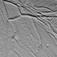
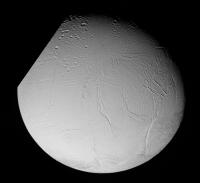
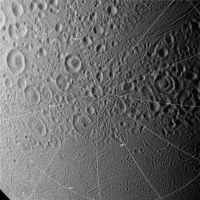
This is the Cassini image I used for the highest resolution part of the DEM:
|
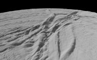
And a single frame from the animation showing a part of this terrain:
|
The DEM should be fairly accurate - in particular the animation should give a very good general idea of what Enceladus looks like even though some details are inaccurate. Also a higher resolution DEM is really needed for these low altitudes - the surface should look less smooth than it does here. Most of the striping is real though as there are lots of parallel ridges and grooves on Enceladus. There may be some spurious stripes but these are very subtle - the obvious ones are real.
I'll do a new animation once I have a significantly bigger DEM. It will probably have better optimized illumination. Shadows are really needed in the first half of this one because I optimized the illumination for the highest resolution part of the DEM. We fly over that part of the DEM at roughly 00:30.
EDIT: To play the animation you need to have an H.264 codec installed (if you are using Windows you can find one http://www.google.is/url?sa=t&source=web&cd=2&ved=0CB8QFjAB&url=http%3A%2F%2Fsourceforge.net%2Fprojects%2Fx264vfw%2Ffiles%2Fx264vfw%2F22_1629bm_23430%2Fx264vfw_22_1629bm_23430.exe%2Fdownload&ei=UWpITKqbAoX94AaJ8vm8DA&usg=AFQjCNEPHJwTszIm24w696DxJbgM7Cgo-w for example).
Posted by: charborob Jul 22 2010, 03:47 PM
I must be missing something in my version of Quicktime because I can't play your .avi file. I'll try to fix that. In the meantime, can you tell me how much vertical exaggeration you have in your rendering?
Posted by: Bjorn Jonsson Jul 22 2010, 03:55 PM
I forgot to mention that to play the animation you need to have an H.264 codec installed (if you are using Windows you can find one http://www.google.is/url?sa=t&source=web&cd=2&ved=0CB8QFjAB&url=http%3A%2F%2Fsourceforge.net%2Fprojects%2Fx264vfw%2Ffiles%2Fx264vfw%2F22_1629bm_23430%2Fx264vfw_22_1629bm_23430.exe%2Fdownload&ei=UWpITKqbAoX94AaJ8vm8DA&usg=AFQjCNEPHJwTszIm24w696DxJbgM7Cgo-w for example).
There is no vertical exaggeration but the true vertical range was rather difficult to estimate accurately. I ended up repeatedly adjusting it until the rendered images approximately matched Cassini's images when using identical illumination and viewing geometry.
Posted by: Floyd Jul 22 2010, 06:16 PM
Very nice! And thanks for the directions to the codec. When I first just tried to open it, my Real player tried but fiailed. When I saved it and opened with Windows Media player all went well.
Posted by: lyford Jul 23 2010, 12:46 AM
Beautiful - thank you!
Posted by: nprev Jul 23 2010, 01:59 AM
 ...outstanding, Bjorn, thank you!!!
Posted by: Ian R Jul 23 2010, 03:43 AM
Very well done!
Posted by: JohnVV Jul 23 2010, 09:41 AM
very nice
it is time consuming isn't it
by the way what program are you using to make the vid .
Posted by: Bjorn Jonsson Jul 23 2010, 07:18 PM
Yes, finishing the DEM is time consuming - it's going to be a lot of work (I'm not even sure I'll finish it this year).
The individual frames are rendered using software written by myself and then assembled into an AVI file using VideoMach.
Posted by: Bjorn Jonsson Apr 19 2011, 02:10 AM
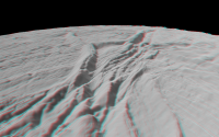
After seeing machi's anaglyphs of Titania I decided to see what an anaglyph of my Enceladus DEM looked like - actually my first ever anaglyph. This first experiment turned out way better than I expected so here it is:
|
Now I really want to do an anaglyph animation of Enceladus.
Posted by: machi Apr 19 2011, 11:27 AM
Very nice!
I'm glad, that my work is inspirational. 
"Now I really want to do an anaglyph animation of Enceladus."
That would be really wonderful and I think, it would be first such Enceladus' animation.
Posted by: Phil Stooke Apr 19 2011, 03:14 PM
Right... approaching the south pole with the plumes rising above the horizon, and then weaving between the plumes... cool!
Phil
Posted by: Bjorn Jonsson Apr 20 2011, 11:06 AM

This would be cool once I have finished a DEM of the south polar region (I'm working on a global DEM of Enceladus). The DEM I currently have is near the equator only.
And here we go, an anaglyph animation of a Enceladus:
encel_anaglyph_xvid.avi ( 2.16MB )
: 692This is the same general area as in the earlier animation but the flight path is different and shorter (the altitude is constant at ~25 km). Needless to say you'll need red-blue glasses to view this properly.
Posted by: machi Apr 20 2011, 12:29 PM
Superb work!
Can you make this animation in reverse direction (opposite view, from flat terrain to mountainous terrain) and approx 2× slower (it's so nice and so quick )?
Posted by: Bjorn Jonsson Jun 28 2011, 08:46 PM
As I have mentioned, I'm working on a DEM of Enceladus using images from the http://pds.jpl.nasa.gov/. Using these images can result in considerably higher quality than using the raw JPGs. This is a by-product of the DEM processing, a 12 frame mosaic of images obtained during Cassini's first close flyby of Enceladus back in February 2005:
|
North is up. This is the first Cassini image product where I used http://isis.astrogeology.usgs.gov/ to a significant extent - for the processing I used various software including ISIS, Photoshop and software written by myself. I used ISIS mainly for correcting the camera pointing angles (this turned out to be suprisingly easy to do once I got past some initial problems using ISIS). The more accurate pointing makes it easier and faster to get the images properly aligned and also yields more accurate results. Soon I should also have a DEM of most of this terrain (the main exceptions are terrain near the terminator and near the limb).
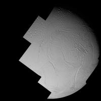
And here is a wide angle context image:
|
I may post more image or mosaics here later. Needless to say, anyone is welcome to post Enceladus-related PDS work here.
Posted by: volcanopele Jun 28 2011, 10:23 PM
Not bad, not bad at all. You did better at blending the high res frame in with the rest than I did:
http://www.ciclops.org/view/2456/Enceladus_Trailing_Hemisphere
Posted by: Ian R Jul 1 2011, 04:09 PM
That's top-drawer, Bjorn. Simply top-drawer.
Posted by: machi Jul 1 2011, 06:26 PM
Feast for the Eyes! 
Posted by: tedstryk Jul 2 2011, 03:05 AM
Wow...Bjorn, that is all I can say, wow. Great work!
Posted by: ElkGroveDan Jul 2 2011, 03:35 AM
Bjorn knows more than a little bit about ice.
Posted by: Bjorn Jonsson Jul 3 2011, 11:24 PM
Yes, a bit
.Regarding Enceladus, more mosaics are coming in the next several weeks, possibly better than this one. And the DEM I now have of most of the terrain visible in the mosaic I posted turned out awesome - I even managed to confuse a rendered image with a Cassini image for a few seconds, the first time this has happened to me. Needless to say I was happy.
BTW ISIS is turning out to be easier to use than I had expected. I used ISIS 2 a bit several years ago but ISIS 3 (which I'm using now) is considerably easier to use in my opinion.
Posted by: elakdawalla Jul 4 2011, 02:13 PM
Are you using ISIS on a Mac or running Linux?
Posted by: Bjorn Jonsson Jul 4 2011, 02:17 PM
Linux on a machine with a dual boot configuration (Windows 7 and Linux).
Posted by: djellison Jul 4 2011, 02:21 PM
On a Mac, apart from having to use the terminal to set some path variables before you use it - it's actually fairly easy. You can run it all from the terminal ( Mac version of a dos prompt ) or you can have actual programs for each app in turn.
Posted by: ugordan Oct 5 2011, 05:26 PM
Calibrated NAC RGB view of Enceladus from Nov 30, 2010:
http://www.flickr.com/photos/ugordan/6209087320/sizes/o/in/photostream/
Posted by: machi Oct 5 2011, 06:53 PM
Beautiful!
Posted by: Phil Stooke Oct 5 2011, 09:01 PM
agreed!
Phil
Posted by: ngunn Oct 5 2011, 10:23 PM
An all time classic. That deserves wide circulation.
Posted by: ugordan Oct 5 2011, 10:36 PM
Thanks.
BTW, if that image looks slightly "foggy" to you, it's not an imaging artifact, it's the dense bulk of E ring around the moon revealing its presence. If Enceladus happened to split the ring optical density along Cassini's line of sight precisely in half, you would expect the background beyond Enceladus' dark limb to be twice as bright as the foreground. Here it's not quite that, but reasonably close. A rough measurement shows the foreground portion at about 60-ish percent brightness of the background.
Posted by: Stu Oct 5 2011, 11:21 PM
Absolutely beautiful. Seriously, why your images aren't *everywhere* - in books and magazines, and on NASA's own websites - is a mystery to me.
Posted by: djellison Oct 6 2011, 12:41 AM
Yeah, someone should do something about that.

Posted by: eoincampbell Oct 6 2011, 02:09 AM
Wondrous !
Posted by: ugordan Oct 10 2011, 08:33 PM
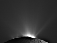
Subject: Enceladus plume temporal variance. 3 NAC clear frames taken roughly at 50 second intervals, unsharped and contrast enhanced:
|
Can you pick up material from a couple of vents going up in "puffs"? I don't think this can be explained by parallax/rotation, the observed rotation of Enceladus is too small for that. I strongly believe this is a genuine variation in output flux on a timescale of a minute.
Posted by: ugordan Oct 10 2011, 08:43 PM
Here's a ratio flicker gif. First frame is frame #2 divided by #1, second frame is frame #3 divided by #2. Shows subtle change in plume appearance from one frame to another better.

|
Notice alternating dark/bright clouds in the plume to the left and to the right. At least two distinct puffs seem to be present in each plume. There's a hint of variation in a third plume at around 12 o'clock but it's much less convincing than these two.
I tried to do a (very) rough measurement of the displacement in the right hand plume during the 50-ish seconds between snapshots and I got a radial velocity of ~250 m/s. I haven't double-checked this. In reality the flow is not in the viewing plane so any number would probably underestimate the real speed.
I've been looking to see if anything like this could be noticed in past plume images and I don't recall seeing anything convincing before.
Posted by: ngunn Oct 10 2011, 09:01 PM
I'm not sure if it's two variable vents or just one that is changing direction, but yes, I agree there is real variation there. A nice obsevation! It's easy to believe - there's no reason why they shouldn't be variable. Perhaps the vent has an ice boulder stuck in its throat. Even in the absence of a mobile obstruction rapid flow is often accompanied by instability/turbulence. I wonder if it has a regular periodicity? Maybe it's singing a low lunar note.
Posted by: machi Oct 10 2011, 10:08 PM
Can you pick up material from a couple of vents going up in "puffs"? I don't think this can be explained by parallax/rotation, the observed rotation of Enceladus is too small for that. I strongly believe this is a genuine variation in output flux on a timescale of a minute.
It's very interesting, but I think, that it's game of shadows.
Posted by: eoincampbell Oct 11 2011, 02:49 AM
Has the long shadow been explained?
Posted by: john_s Oct 12 2011, 02:34 AM
Awesome find! It looks pretty convincing to me.
Congratulations Gordan!
John
Posted by: nprev Oct 12 2011, 10:22 PM
Re the long shadow: Looks to me like that's probably an effect of the shadow of Enceladus itself; parts of the plumes are in sunlight, some aren't. There are other plumes in the foreground of the shadowed region, which makes it look a little weird but that's a perspective effect.
Posted by: hendric Oct 13 2011, 06:24 PM
Isn't that mostly Saturnshine lighting up the surface? It looks like the rightmost pixels are blown out, so that's where the sunlight terminator is located. The multiple shadow-lines are caused by the mostly-linear nature of the plumes; the further ones are more "down" I guess.
Posted by: Bjorn Jonsson Nov 15 2011, 09:54 PM
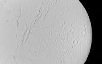
This is a 21 frame mosaic of images obtained during Cassini's targeted flyby of Enceladus back in March 2005:

|
North is up and the resolution of the images I used ranges from ~35 m/pixel to ~350 m/pixel. This image is actually a by-product from a different image processing project; I should soon have a shape from shading DEM of most of this terrain.
The images were reprojected to simple cylindrical projection. The resulting map was then rendered with subspacecraft latitude=-1.4 and longitude=203.8 without applying any illumination.
Processed using mainly a 'mix' of ISIS, Photoshop and software written by myself.
Posted by: Juramike Nov 16 2011, 01:02 AM
Wow! The detail in that image is fantastic! Bravo!
Posted by: tedstryk Nov 16 2011, 05:59 PM
I saw it and thought, "Oh, that's pretty." Then I zoomed in- AMAZING!!!
Posted by: Guillermo Abramson Nov 17 2011, 01:37 AM
Amazing. Thanks for sharing it.
Guillermo
Posted by: dilo Feb 8 2012, 09:19 AM
Congratulations to Gordan for today's APOD mosaic, it is really stunning!
http://apod.nasa.gov/apod/ap120208.html
(I would like to see more in the plume region but I guess wasn't photographed).
Posted by: ugordan Feb 9 2012, 11:27 AM
http://apod.nasa.gov/apod/ap120208.html
(I would like to see more in the plume region but I guess wasn't photographed).
Thanks, but that doesn't really belong to this thread. The image (not a mosaic) was taken a year ago.
Thanks for pointing this out. Posts moved to the correct thread - moderator
Posted by: scalbers Feb 25 2012, 06:07 PM
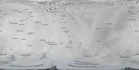
Greetings - thought I'd post my latest Enceladus feature map here:
|
(Note to mod, technically this includes some PDS and older raw images, so the best thread/forum for this might be considered)
Posted by: elakdawalla Feb 26 2012, 10:18 PM
These are cool, Steve! Thanks for sharing. Regarding where they should be put -- the point of the "raw" threads is to discuss ongoing mission in real time (the way the MER threads work), "PDS" threads are about manipulation of data sets. You've posted in the right place.
Posted by: scalbers Feb 27 2012, 07:51 PM
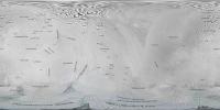
Thanks Emily. Here's an updated version where more of the feature labels are rotated and offset for the Dorsa, Fossae, Sulci and such...
|
Full Resolution here: http://laps.noaa.gov/albers/sos/features/combined_enceladus_lon_180_center.png
That's the latest,
Steve
Posted by: Bjorn Jonsson Mar 4 2012, 08:14 PM
My latest animation:
http://vimeo.com/37689757
This is an almost 7 minute animation featuring a digital elevation model (DEM) covering roughly 50 percent of Enceladus' surface. It is the most complex and by far the biggest animation I have ever done. The DEM is created from 55 of the images Cassini obtained during its three close flybys of Enceladus back in 2005. The flight path, viewing and illumination geometry is carefully selected to completely hide the fact that the DEM is not global. The DEM's resolution varies from ~70 to ~350 m/pixel. The field of view is 50 degrees.
The DEM is created using a very simple shape from shading algorithm (SFS) followed by 'destriping' and extensive post processing. A significant amount of the processing is based on (or some processing ideas were indirectly triggered by) various tips posted in several threads here (in particular, some of JohnVV's posts were helpful). All of this processing was done using a mix of ISIS 3, Photoshop and software written by myself. The individual frames were rendered using a renderer written by myself. The first frames were rendered in early December but due to the size of the DEM and this animation project several things have changed since then. The most significant change is that I finally built a 64 bit version of the renderer in early January (the DEM is too big to be easily manageable at close range using the old 32 bit version).
Since the DEM is created using SFS, vertical exaggeration is variable across the DEM. I tried to keep it uniform and close to 1 but this really is impossible to do accurately without combining the SFS DEM with another DEM created using stereo imaging. A lot of stereo coverage is available but I haven't done this yet since it takes a lot of time - I may do it later. Vertical exaggeration probably tends to be greater in the highest resolution patches than in the lower resolution areas. It should be noted that for Enceladus I used a uniformly white texture map, i.e. all of the details visible are from the DEM. Compared to the source images, resolution loss is minimal in the DEM.
There is probably sufficient medium to high resolution data available to make a global DEM with one exception: The north polar region. Hopefully Cassini manages to completely image the NPR at 300-500 m/pixel (or better - preferably 100-300 m/pixel) later in its mission.
A few sample frames:
|
|
|
|
Needless to say I recommend fullscreen viewing (and a biased comment: Looks awesome on a large TV screen).
Posted by: scalbers Mar 4 2012, 08:38 PM
Very nice animation Bjorn. It's fun to try and recognize various features as you fly over. One example is the sequence starting at 4:55 when the crater Sabur is centered in the view. Then from 5:00 to 5:12 we are flying northbound alongside Anbar Fossae. At 5:21 we're transitioning from Samarkand Sulci to Hamah Sulci (note unnamed crater at that time), then about 5:30 when flying from Hamah Sulci down to Ebony Dorsum.
Earlier at 2:23 we come upon a double crater, the one on the right side being Al-Mustazi. We approach the northern part of Bishangarh Fossae at 2:26. Then we catch the western part of Al-Yaman Sulci (oriented from left to right) around 2:33. By 2:43 we swing to look at the southern end of Harran Sulci (towards the west). At 2:49, we are looking westward at the northern end of Khorasan Fossa. At 3:00 we spot the intersection of Harran Sulci and Kaukaban Fossae near the limb. Then by 3:07 the crater Harun is located above the center. The southbound canyon fly through at 3:30 looks like we're going back through the southern end of Harran Sulci.
Perhaps the makings of a narrated sound track?
Things like the serrated limb help to make this look very realistic. Might be interesting to consider texture and even some slight color at some point?
Steve
Posted by: ugordan Mar 4 2012, 08:47 PM
On the contrary, I think Bjorn nailed the color here.

Interesting to watch the phase angle effects as well, it's clear right from the initial frame that the photometric modelling of the disc is more realisic than what one would expect from just illuminating a ball in a commercial 3D renderer. About the only thing that gives away the fact this is a rendering is the lack of secondary illumination of shadowed slopes near the terminator by the opposing sunlit slopes. Other than that, add some point spread function and this could pass under an actual Cassini image.
Posted by: machi Mar 5 2012, 10:21 AM
It looks fantastic Bjorn!
Can you make some anaglyph versions?
Posted by: Bjorn Jonsson Mar 5 2012, 10:10 PM
[snip]
Perhaps the makings of a narrated sound track?
Things like the serrated limb help to make this look very realistic. Might be interesting to consider texture and even some slight color at some point?
Steve
A narrated sound track - that's an interesting idea. And it's nice to see there are lots of recognizable features there ;-). Regarding texture, it wouldn't add any details since compared to the original images, loss of resolution is negligible in the DEM.
I'm using a slightly modified version of the earliest Hapke function - it's modified to avoid unrealistic effects when the emission angle approaches 90 degrees. The phase effects are interesting and very strong. I even had to reduce the opposition effect a bit to avoid problems with dynamic range.
The lack of completely black shadows (no secondary illumination) is a problem and makes terminator closeups less realistic. The only reason I avoided them was to speed up the rendering time. Adding a point spread function is a nice idea but some of my test renders look realistic to me anyway. A year or two ago I somehow managed to confuse an Enceladus test render with a Cassini image for a few seconds. Needless to say I was happy when I realized what had happened.
Can you make some anaglyph versions?
That's probably a bit complicated due to the complicated flight path. A bigger problem is rendering time even though my renderer is at least two times faster now than it was two months ago. But this might be an interesting future project.
Posted by: JohnVV Mar 6 2012, 06:24 AM
nice
It might be my imagination but
did you use ISIS to " destripe "
I have been reprocessing the venus data and have been seeing that X cross hashing every where
Posted by: Bjorn Jonsson Mar 6 2012, 11:44 PM
I used ISIS' dstripe 'indirectly' - the dstripe documentation contains a fairly detailed description of the algorithm used to destripe and this enabled me to implement this capability in my own software. I've mainly been using ISIS to correct the camera angles (jigsaw, deltack etc.).
Regarding the "X cross hashing" - if this is what I think it is I've seen it too. I've found that fairly often after I destripe, new narrow and fainter stripes appear that have an orientation that differs from the orientation of the original stripes. When this happens I need to rotate the DEM (to make the new stripes horizontal), destripe again end rotate the DEM back. Sometimes I need to do this several times. Sometimes this is a prolonged trial and error process.
Posted by: Zack Moratto Mar 9 2012, 10:44 PM
Do you have a list of stereo pairs that could be processed? ISS images usually process pretty quickly in ASP and would make a fun test case for me. I could then share my results back to you via this thread.
Posted by: Bjorn Jonsson Mar 10 2012, 01:34 PM
Not a list but the March and July 2005 flybys provided lots of stereo coverage since there is a lot of overlap - the March flyby was equatorial and the July flyby south of the equator with the illumination geometry almost identical.
Stereo pairs from these flybys are easy to find - one example is images N1500059045_2.IMG (July) and N1489045316_2.IMG (March).
There is also stereo coverage from later flybys but I'm not yet familiar with the details of these flybys.
Posted by: PDP8E Mar 10 2012, 05:14 PM
Bjorn,
That flight was tremendous! Thanks for sharing your hard work.
You and your work are an inspiration.
~pdp8e
Posted by: Ian R Mar 11 2012, 08:47 PM
I'll second that.
Posted by: FordPrefect Mar 13 2012, 01:01 AM
Outstanding video Bjorn! Amazing!
I loved the phase-angle effects too. Could you elaborate on the modified version of the earliest Hapke function or point to where that function can be found? Those zero-phase glares are very prominent on the Moon/lunar surface too, but I suspect generally on any body with rough surfaces.
Thank you very much for any pointers!
Edit: Is this what you've been working with? -> http://selena.sai.msu.ru/Pug/Publications/ms42/m42_60.pdf
Rafael
Posted by: Bjorn Jonsson Mar 17 2012, 12:47 AM
The modified Hapke function I'm using can be found in my software and (probably) nowhere else ;-). What I'm doing is a crude (probably), simple and empirical modification: I'm preventing the emission angle from ever getting 'too close' to 90 degrees by multiplying it with a number that is a slightly lower than 1 once the emission angle exceeds ~80 degrees. This number is actually a function of the emission angle and gets a bit lower as the emission angle approaches 90 degrees. This may seem strange but since the patch of surface within a pixel really is never perfectly smooth the average emission angle of the visible 'facets' within the pixel should never get extremely close to 90 degrees. This is simpler (but also less accurate) than the more complicated forms of the Hapke functions and eliminates unrealistic bright 'rims' around some terrain edges or planetary discs.
Posted by: FordPrefect Mar 17 2012, 01:58 PM
Thank you very much Bjorn for the insight!
Posted by: Bjorn Jonsson Nov 5 2017, 08:10 PM
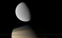
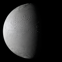
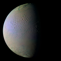
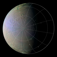
On November 27, 2016 Cassini at last obtained really good images of Enceladus' north pole during a nontargeted flyby. This is a mosaic of two IR3-GRN-UV3 color composites processed to show Enceladus in approximately natural color and in greatly exaggerated color which reveals compositional variations. A version with a latitude/longitude grid is also included.
|
|
|
The images comprising the mosaic were obtained at a range of 62,000 to 72,000 km. ISIS3 (qnet/jigsaw) was used to correct the camera pointing. I then reprojected everything to simple cylindrical projection and rendered the images using software I wrote. The final step was to use Photoshop to process the color.
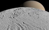
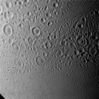
The highest resolution view of the north pole obtained during this flyby is a clear filter image at a range of 32,000 km. The resolution is 190 m/pixel:
|
|
Posted by: jccwrt May 24 2018, 09:17 PM
Monochrome image mosaic of Enceladus taken during the targeted E10 flyby, at a distance of 40,000 km
https://flic.kr/p/27ta96Dhttps://flic.kr/p/27ta96D
IR3, GRN, UV3 extended color mosaic taken a little closer, from a distance of ~20,000 km.
https://flic.kr/p/27p1hpAhttps://flic.kr/p/27p1hpA
Both mosaics primarily target the equatorial regions of the leading hemisphere between about 200E and 0E.
Powered by Invision Power Board (http://www.invisionboard.com)
© Invision Power Services (http://www.invisionpower.com)