Juno, perijove 12, April 1, 2018 Options

[Gerald]

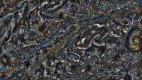
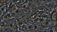
Here is a europlanet press release about our ProAm Juno meeting a few days ago:
"New views of Jupiter"

Of course my main talk has been only one among several contributions. But Anita Heward, who has written that excellent press release, was especially interested in highlighting Seán's and my JunoCam image products. So, I provided her some of my crazy attempts to infer a vector field of displacements from a pair of reprojected, cropped, contrast-normalized, and heavily enhanced PJ12 JunoCam images.

Besides Seán's latest masterpiece of merging, cleaning, and enhancing some of my reprojections, you'll find an animation, together with a link to an according MP4, in the above article, if you scroll down a bit. It extrapolates one of the two images 100-fold into the past, and into the future, with respect to the time span between the two original images. The morph is an integration assuming a stable velocity field. It's calculated via numerical integration of the numerically given differential equation using probably the simplest-known method, called Euler method. I've subdivided either integration into 1,000 equal steps, such that I expected the numerical error being considerably smaller than the statistical and systematic errors, despite the slow convergence behavior of this method.
In order to avoid artifacts induced by regular grids, I've applied Monte Carlo methods whenever I had a choice within the short preparation time.
My full talk considered derivatives like curl, divergence, or the Laplacian, as well as the effect of statistical errors induced by the choice of the actual Monte Carlo samples for stereo correlation.

I might be able to upload the according MP4 (without audio, 630 MB) next weekend, and provide an according link.

[fredk]

Congaratulations guys on all this work.

I'm curious, Gerald, which DE did you solve?

[Gerald]

Thanks!
The displacement field derived by stereo correlation, and smoothed by a bandpass filter represents a numerical description of a vector field, such that numerical integration methods for differential equations can be applied, especially solutions of the initial value problem. A morph is essentially such a solution applied to a set of initial values.
At this level of elaboration, the displacement field is just a vector field of pixel displacements, i.e., the displacement is a function of pixel position, however not yet of an immediate physical meaning due to the neglected projection between image coordinates and physically more meaningful coordinates. The differential equations are also only given numerically and implicitely in terms of displacement fields, although some of the derived entities are related to the Navier-Stokes equations.
Especially, I've made some experiments with the Lamb vector and its first derivative, in order to get an idea, whether a verification of the Navier-Stokes equations might be feasible, or where the velocity field is consistent with the assumption to be irrotational.
Like Anita has written, those are feasibility tests that give a qualtitative idea, not yet final physically calibrated and fully interpreted results.

[Sean]

PJ12_81 using Brian Swift's pipeline...



*edit: fixed link*

[Gerald]

YouTube upload of the visuals of my #RASJuno talk in London last week is completed.
And here the original full HD version of about 630 MB.

[Bjorn Jonsson]

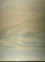
Better late than never; here is an image I processed some time ago from PJ12_90:



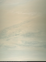
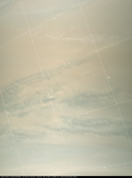
This image has been specially filtered and enhanced to increase the visibility of the mesoscale waves that are present in the pale orange Equatorial Band (EB) within the Equatorial Zone (EZ). Many of waves appear rather subtle if no processing is applied. Bright clouds are also visible near the top of the image. To avoid 'saturating' the bright clouds, the processing of the area containing these clouds differs from the processing elsewhere in the image (in particular, more 'gentle' filtering was used).

Here is an approximately true color/contrast version:



Because of the viewing geometry and the wide field of view the image has some perspective foreshortening. Below is the approximately true color/contrast version with a latitude/longitude grid. Latitude is planetographic.



As the latitude/longitude grid implies, the image covers a very small area on Jupiter. A global context view shows this better. It is based on Marco Vedovato's map that includes images from March 29-31, 2018. All of the PJ12_90 observation is shown but the white box shows the extent of the images above:



And finally some metadata:

IMAGE_TIME = 2018-04-01T09:52:02.073
MISSION_PHASE_NAME = PERIJOVE 12
PRODUCT_ID = JNCE_2018091_12C00090_V01
SPACECRAFT_ALTITUDE = 4726.4
SPACECRAFT_NAME = JUNO
SUB_SPACECRAFT_LATITUDE = -2.6206
SUB_SPACECRAFT_LONGITUDE = 120.2951
TITLE = Equatorial Zone
Resolution at nadir: ~3.3 km/pixel

[Gerald]

For these suble to very subtle features, and for a few other purposes, I've implemented kind of a hipass filter that considers local contrast as well as validity of data.
Here a link to a cylindrical map projection of PJ12, #90 (about 55 MB, 3600x7200 pixels PNG) that averages the hipass-filtered image with an illumination-adjusted and gamma-enhanced version, in order to recover some global colorization.
Rendering large maps with this filter takes several hours, however.

Scroll down to the center and a little further below for the mesoscale waves. There are also some more subtle waves above the center, as well as a second diagonal of wind-blown "popup" clouds, maybe some kind of cirrus, like cirrostratus.

[fredk]

solutions of the initial value problem

Sorry, Gerald, I finally looked at those results. It's still not clear exactly what DE you solved. Perhaps you estimated the curl of the initial 2-frame displacement field, and then somehow evolved the field with the constraint that the curl remain constant? So vortices remained localized?

It looks like you also considered the divergence of the initial field, though on physical grounds I guess that should be small in the absence of significant up/downwelling. So any nonzero div may be due to noise in the determination of the initial field, and one approach to reduce noise might be to force the div to zero.

I guess you've made no attempt to try to infer physical quantities such as the pressure field?

[Gerald]

What I've implemented has been pretty simple. I just inferred a bandpassed displacement field. This could be interpreted as an approximation of a velocity field. Everything is given only numerically.
More generally, this displacement field can be understood as a field of 1st order tensors, given explicitely.
Each pair (x,y) of the plane is assigned a vector (dx/dt, dy/dt), describing which infinitesimal amount (dx,dy) a vector (x,y) is to be displaced after an infinitesimal time step dt.
Write this assignment as (dx/dt, dy/dt) = f(x,y).
I'd classify this as a first-order partial differential equation.

So. for each pixel position in the image plane, an approximate velocity is assigned. That's essentially the DE, represented only numerically. This DE can be integrated forward, or backward in time. I've implemented both by the Euler method, the most simple numerical method to integrate DEs.
Other than the 1-dimensional case described in Wikipedia, the settings here are 2-dimensional.
And we don't have a time-dependency of the tensor field. It's assumed stable, instead.

All the derivatives are infered numerically from the displacement field (approximate velocity field). They aren't required for the integration of the DE on the above level, but are subject to a separate investigation.
I didn't make assumptions constraining curl, divergence, or Laplace operators, but instead just calculated them numerically from the displacement field. Any assumptions about these operators could be made, but they would define results that should better be determined from the data instead of being presumed. Up and downwelling are well possible and shouldn't be ruled out by assumptions. Even a zero Laplacian may be plausible under idealized conditions. But how can we assume these conditions without trying to measure or infer them? I think, that any unnecessary assumption should be avoided, and we should instead measure and infer everything we can from actual data.
I think, the most significant approach of criticism of the method implemented thus far is the implicite assumption of a stable velocity field. I.e., the integration over the displacement field is assuming, that the displcement field doesn't change over the integration time interval. This simplification, and likely oversimplification, should be verified, at least, or better be refined, by investigating not just a pair of images, but a longer time-series. Such a time series may allow to detect and model changes of the velocity field over time, and result in more accurate particle trajectories than just in flow lines.
Another possibly relevant point is the difficulty to properly determine vectors with a non-zero component normal to Jupiter's "surface", or to the image plane.
Once the numerical representation is fully elaborated, including the reduction to physically meaningful units, this representation can be checked against Navier-Stokes, simplifications to special cases, or extensions.

[Gerald]

... Example:
Start with the image pair

...

[Gerald]

... for each pixel position (x,y), estimate the partial derivatives of x and y with respect to t:

That's a visualization of the numerical description of the DE.

Then integrate over time via an Euler method:
 PJ12_099_100_10000samples_mode2_seed000001_grow.mp4 ( 596.69K ) Number of downloads: 230

(here for some randomly chosen initial values)

[fredk]

Now I see - that is extremely simple. Thanks, Gerald, for the description. So indeed the crucial assumption is of a steady flow, ie constant flow velocity at each point. Indeed looking at more that two frames would help, in at least two ways. First, by giving you a sense of the time dependence of the flow field f(x,y). This could be fitted to simple polynomials or splines to approximate the time dependence (though substantial extrapolation is still risky). But more crucially making several estimates of the flow field would also mean beating down the noise, which has to be large when you only use two frames.

Are there triple or more frame sets that you could use in practice?

My comment about the div wasn't to say you should make that assumption. I think it would simply be interesting to impose div f = 0 and see what difference it makes. A large difference would mean that this is an important consideration and should be investigated further. So it would simply be a test.

[hendric]

It's like https://earth.nullschool.net/ except for Jupiter! Very nifty!

[Gerald]

Yes, thanks! That's indeed the same kind of visualization for the flow lines of Earth's wind field.

Are there triple or more frame sets that you could use in practice?

I guess, that this might be possible closer to the poles. There, we have time series of several images. and may be up to a handfull within a respective series that might be of a sufficient quality to determine velocity fields. During PJ13, for the first time, JunoCam has taken a sequence of TDI 3 images of the south polar region. I think, that those images will be the best basis, thus far, for an attempt to find areas of unsteady flow.

Regarding div, laplace, etc, I've run statistical tests, too, whether the retrieved values are significant, i.e., above noise induced by the choice of Monte Carlo samples used for stereo correspondence. In this repect, all these derived entities appear to deviate significantly from zero, for at least some areas. But there are still statistical errors induced by the structure of the data to be ruled out.

There are various issues to beat down. The first limits I tried to test have been Jupiter's latitude, respectively the time from closest approach. It's the harder to get useful image pairs the closer we get to a perijove. That's due to the very rapid change of perspective. Currently, my limit to get useful results is somewhere near 5 minutes between two images taken from very different perspectives. For the equatorial zone, or later, for the perijove anticipated to migrate towards north, I should push the limits to below two minutes. This requires a very accurate global camera calibration and pointing. Therefore, my primary goal for the next three months is developing families of camera models more suitable for JunoCam calibration than the straightforward Brownian approach.
At the same time, I'll run tests with the south polar PJ13 sequence, in order to be able to provide feedback for planning future flybys (assuming them to take place, and with healthy instruments). One of the tests will include the feasibility of an inference of a displacement field between velocity fields, or at least comparisons between velocity fields derived from image pairs within a sequence of south polar images.
We'll then see, whether or which of those higher-order properties of the velocity field can be determined above noise level.

[Bjorn Jonsson]

Very interesting discussion, thanks for all of this information

Are there triple or more frame sets that you could use in practice?

I guess, that this might be possible closer to the poles. There, we have time series of several images. and may be up to a handfull within a respective series that might be of a sufficient quality to determine velocity fields. During PJ13, for the first time, JunoCam has taken a sequence of TDI 3 images of the south polar region. I think, that those images will be the best basis, thus far, for an attempt to find areas of unsteady flow.

There are some Voyager triple frame sets where the interval between frames is ~30 minutes if memory serves. It would be interesting to try something like this on these frame sets.

(and now I have yet another reason to be unhappy that Galileo's HGA didn't work...)