MSL data in the PDS and the Analyst's Notebook, Working with the archived science & engineering data Options

[Gerald]

Planck's function isn't linear, and it's dependent of the absolute temperature. So it should be possible to infere the absolute temperature from the brightness temperatures at two known wavelengths and two different temperatures...
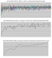
Under ideal conditions, in theory.
Before doing theory in detail, I first checked the data to find out, whether it can work in practice.
The intermediate answer is: Not in a straightforward way.
Emissivity seems to change with time, and in a different way for the two frequency bands A and B.
The first reason I could isolate is warm-up. Here some statistical analysis of 18 warm-ups on sol 89 for brightness temperature A, based on this Sol 89 REMS RDR file:


The first diagram shows brightness temperature A for the first 100 seconds of 18 warm-ups, adjusted by average and stretched by respective standard deviations.
The second diagram averages over these 18 curves.
The third diagram smoothes the latter curve by averaging over a window of 10 seconds.
It shows a significant average increase of brightness temperature A during warm-up.

So a first step to get better data, will be to apply the last column (column 63) of the referenced table, indicating warm-up, not just to pressure data as described in this FMT file, but also to brightness temperatures.

EDIT: Some number-crunching later: Radiance at 250K and 11um seems to be much less (about factor 5) sensitive to emissivity near 1 than to absolute temperature (use Planck function with 250K at 11um as brightness temperature, and divide it by the value at 255K as absolute temperature; the result is the corresponding emissivity). So an emissivity of 0.9 will lead to an absolute temperature 5K above brightness temperature (near 250K). I overestimated emissivity in the beginning. Although I didn't yet investigate, how the emissivity quotient influences measurement of absolute temperature by dividing radiances of two wavelength bands (two-colour pyrometer).

[Gerald]

Here the simplified theoretical principle for the two-colour pyrometer to calculate absolute temperature and the emissivities at two wavelengths from brightness temperatures, as far as I could infere it from Planck's law:

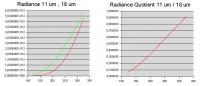
Input data: Take the (measured) brightness temperatures Tb_11 and Tb_18 at two frequencies nu_11 = c/11um and nu_18 = c/18um.

Algorithm:
Apply Planck's function to retrieve measured radiances I_11 := I(nu_11, Tb_11) and I_18 := I(nu_18, Tb_18).
The graph of the according Planck functions is shown in the left of the two diagrams:


Now start an iteration with initial emissivities E_11 = E_18 = 1:
Calculate a modified radiance quotient by Q := (I_11 / E_11) / (I_18 / E_18).

Calculate absolute temperature T_abs := T_abs(Q) for a given radiance quotient Q by applying the inverse function of the quotient I(nu_11,T)/I(nu_18,T) of the Planck functions (restricted to an appropriate temperature interval).
The graph of I(nu_11,T)/I(nu_18,T) is shown in the right of the two diagrams above.

Apply the Planck function to T_abs, to get the black body radiances I(nu_11, T_abs) and I(nu_18, T_abs) at T_abs for nu_11 and nu_18.
Calculate E_11 := I_11/I(nu_11, T_abs) and E_18 := I_18/I(nu_18, T_abs) to get better approximatives for the emissivities.
Repeat the iteration until T_abs changes less than a given epsilon; abort with an error, if it doesn't converge after an upper bound of iterations.

If the iteration converges, we get absolute temperature, and emissivities at both wavelengths.

[jmknapp]

Have you tried this on the time series yet? In one of the press conferences they had a chart of ground temperature vs. time that could be used as a rough check. Another issue would be how best to deal with the noisy raw data.

On the "warm up" effect--what does that refer to exactly? Like when the readings are taken after an idle time of an hour or so? Looks like they normally take readings every second for a few minutes every hour, with occasional longer stretches.

[Gerald]

I'll answer the easy questions first:
Most of the noise can be averaged away by appropriate low-pass filters, if it is purely statistical, because temperature changes are slow; the simplest way to do it, is just averaging over a few dozens of samples; a more advanced way is using appropriate regression curves.
Example for simple averaging over 40 samples:

Again based on this Sol 89 REMS RDR file.

About warm-up I know just that little info from the FMT-file; it referes to pressure data:

OBJECT = COLUMN
COLUMN_NUMBER = 63
NAME = "PS_CONFIDENCE_LEVEL"
DESCRIPTION = "String representing the confidence level for the
pressure sensor; 0 = bad; 1 = good;
- Byte 0: Warm up effect (only for barocap 1)
0 = warm up effect; 1 = no warm up effect;
- Byte 1: Shadow effect; 0 = shadow effect;
1 = no shadow effect;"
DATA_TYPE = CHARACTER
START_BYTE = 568
BYTES = 8
END_OBJECT = COLUMN

Warm-up seems to take 180 seconds at the beginning of each series of measurements, at least on sol 89.

[Gerald]

Have you tried this on the time series yet? In one of the press conferences they had a chart of ground temperature vs. time that could be used as a rough check.

The simplified answer is: No, not yet, but a good idea for a better calibration.

A little more detailed: I also looked at the UV data. They are less noisy. I tried to get a 5-point absorption spectrum of atmospheric trace gases, that form or degrade after sunrise. For this I had to do a very detailed analysis. Doing this, I also found a jiggering caused by truncation of numeric values, and indications for superposed sinus oscillations with a period of about 300 to 350 seconds of unknown origin, might be due to my way of data analysis, may be due to data analysis done by the REMS team, or due to technical properties of the sensors, like a combination of inductivity and capacity.
Similar systematic errors may also occur for brightness temperature data. Accurate results for absoute temperatures can only be obtained, after those systematic effects are annihilated. Therefore I was focussed on that.
The only thing I had been doing, was dividing the Sol 80 EDR raw thermopile A/B data to see, whether they can be used as two-band pyrometer data, and it looked good, but calibration wasn't available to me.
It will take me a while to elaborate things in more detail.

[Gerald]

Here the sol 89 results, based on the two-color pyrometer algorithm described above, and the Sol 89 REMS RDR data, without correction of systematic errors, no bugs assumed:

The green curve in the top diagram describes the inferred absolute Kelvin temperature by record (not by time), averaged (all weights set to 1) over 40 samples.
Absolute temperature was restricted to a range between 100 and 400K before averaging.
The bottom diagram describes the inferred emissivities, also averaged over 40 samples.
Emissivities were restricted to a range between 1e-20 and 100 before averaging.

The algorithm leaves one degree of freedom, e.g. the emissivity quotient. It is set to 1 in this run, meaning grey body assumed.

The absolute emissivity values look rather confusing to me, because I expected them to be between 0.9 and 1.0, and constant over time.
On the other hand, absolute temperature values look rather reasonable for less noisy regions (sufficiently high brightness temperatures).

Any of my attempts to get more reasonable-looking emissivities by adjusting emissivity quotients, absolute value of one of the emissivities, or wavelengths failed,
because other values became less reasonable.

Some calibration of the absolute temperature is possible by adjusting the difference of the wavelengths.

[Gerald]

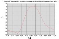
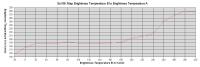
In one of the press conferences they had a chart of ground temperature vs. time that could be used as a rough check.

The best approximation of the chart of the press conference I could get, was just using Brightness Temperature A of this Sol 10 REMS RDR Tab File, discarding 180s warm-up at the beginning of each measurement, and averaging:

Compare it with http://photojournal.jpl.nasa.gov/jpeg/PIA16081.jpg.

[PaulH51]

Gentlemen,

Not sure if you are aware, but the Spanish REMS team (Ashima Research) have "processed" the 1st 90 days of the REMS data using the public NASA PDS data sets.

Their page provides NetCDF versions of the first 90 sols of REMS measurements created from data available in public PDS archive as of March 20th, 2013. Each file is a direct conversion from the PDS archive of the corresponding file type (except for the ADR files, which is now split into two files containing the correction and geometry data, respectively. 'UNK' data values are converted to masked data, -9e36 for floating point, -2**15 for integer.

Each variable in the PDS dataset is converted to a NetCDF variable depending on the type stored in the PDS label .CHARACTER variables (strings) are converted to character arrays, ASCII_INTEGER to 32 bit integers, ASCII_REAL to 32 bit floats. In addition a "Time" dimension is added by dividing the TIMESTAMP data by 86400 to give the number of days since noon January 1, 2000. The Local Mean Solar Time (LMST) stored in the PDS tables is stored as a 18 character string, and split into sol, hour, minute, and second, with the latter containing the milliseconds component. Where available, the unit and description fields for each column have been converted to NetCDF variable attributes.

I hope that this will assist in resolving some of the issues you have encountered, but will no doubt raise further questions and additional debate

LINK to page containing the document download links : http://www.marsclimatecenter.com/rems.html

LINK to Blog post that alerted me of this data : http://marsweather.com/first-90-sols-of-re...cessed-versions

[Gerald]

Thanks! This may help more people to access the PDS data, and contribute to the debate.
I personally have been learning how to work with PDS data directly, and how to read and process them with spreadsheet or self-written software.

I think, the underlying question is, how to interprete the REMS data correctly. Several of those questions have been answered during the recent EGU conference, e.g. the origin of the UV oscillations I mentioned before; they seem to be attributed to gravity waves, not to systematic errors as I've been suspecting as likely, surprising news (to me)! Or rover movements leading to changes of the measured area, less surprising, but important to consider.
Difficult to understand are Brightness Temperature B data; jumps in the time series of e.g. UV data still have to be explained explicitely, afaik, most likely recalibrations, imho.

[Gerald]

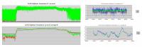
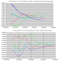
Here one of the charts that shows UV oscillations, which I was assigning to my lack of appropriate data analysis:

It's still based on this Sol 89 REMS RDR file.
The first diagram describes each of the UV curves normalized by its average and divided by the UV ABC value.
The second diagram contains delta curves, obtained by averaging values of 150 seconds and subtracting this from the average of the next 150 seconds of the first diagram.

My original intention was to find a shift of absorption for different UV bands, that might indicate a short-term change of composition of the Martian atmosphere.
(Btw.: A shift between the red curve (UVA) and the green curve (UVB) - the two steeply ascending curves in the first diagram - looks obvious.)

The fine jiggering is likely due to numeric errors.
The next-longer oscillations have been the mystery. Can anyone else duplicate similar results? Are they due to errors or due to real physical processes like gravity waves?

[PaulH51]

I think, the underlying question is, how to interpret the REMS data correctly....

I was sort of hoping that the "Processed Data" would have provided more insight to the well documented issues you and Joe have been debating, I have been following your discussion closely, sadly I do not have the knowledge to contribute. However, I have been learning much as it progresses... So lets hope the provision of the "Processed" REMS data does bring more people into this debate.

Separately I was also hoping that the chart detailing the ground temperature (min / max) for the first 200 sols released at that EGU conference would have helped you and Joe to test / prove some of your theories / assumptions re the temperature of a target by understanding the brightness temperatures.

I will continue to monitor this debate and hopefully learn a lot more along the way...

Thanks

[Gerald]

Thanks for your interest!
There are ways to go deeper into analysis.
First: The emissivity values obtained thus far are most likely nonsensical.
During the conference they told, that kinetic temperature should be at most three Kelvin above brightness temperature. That's exactly my opinion. And it means, that emissivities for both IR wavelength bands should be between 0.9 and 1.0, and rather similar to each other, as stated earlier. Taken this as a basis we get a contradiction to the results above. The logical consequence is, that at least one of the assumptions was wrong.
One assumption was a two-color assumption instead of a two-band assumption in order to avoid calculus.
An other (implicite) assumption was, that noisy temperature data are allowed to be averaged to get the actual mean temperature; this is valid only for symmetric noise distribution.

Both assumptions will most likely to be replaced by more appropriate ones. Dropping the first one might lead to a spectrum combined of the spectra of the two IR sensors and the wavelength-dependent albedo/emissivity properties of the soil.
Dropping the second one may lead to a function, which transforms Gaussian noise to the actual noise. The idea to get this function may be the calculation of the higher momenta of the noise distribution, and infer from this the first few Taylor coefficients of the transformation function; I'll have to check, whether it works in this case. The result may then be used to average appropriately.

There will remain rover- and sun-induced effects that have to be isolated.
I'll explain details based on actual data, as soon as I succeed with one step. It's far from easy, and I've other jobs as well, so it may take a little time.
Everyone is invited to contribute improved solutions.

[Gerald]

A small step towards a better assessment of Brightness Temperature B:
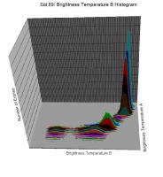
Take a (cartesian) coordinate system with two axes, one for Brightness Temperature A, one for Brightness Temperature B.
Now take the Sol 89 data and add a point for each record of the data at the respective (Brightness Temperature A / Brightness Temperature B ) position.
Tile the coordiante system parallel to the axes. Count the points in each rectangle and take that count as the respective position on a third axes.
The result is a sequence of histograms. They may be drawn in the following way as "slices":

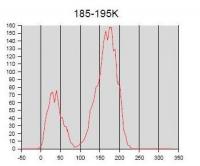
Looking just at one such "slice" (for a fixed Brightness Temperature A interval) at a time, and repeating this for the first 20 slices may result in an animated gif like this one, as a different way to represent the same data:

(Link to the gif)
The headline indicates the considered Brightness Temperature A interval. The horizontal axis describes Brightness Temperature B. The vertical axis shows the number of entries near the respective Brightness Temperature B.
(I allowed neighbouring slices to overlap.)
The diagrams show clearly, that for low Brightness Temperature A there are two peaks for Brightness Temperature B. That's not at all a Gaussian distribution. So the concern about averaging correctly is justified based on actual data.

[Gerald]

The official statement regarding the noise of thermopiles B and C according to the PDS file REMS RDR Data Set Reference Information is

Data from thermopiles B and C of the Ground Temperature Sensor are included but are too noisy to be considered useful.

I'm not yet quite at that point, because the noise seems to be structured; it might be possible - besides appropriate averaging - to exploit this structure by analysing a sufficiently large set of data.
Examples:
1. The double peak of the Brightness Temperature B noise distribution seems to indicate temperatures below 200K. Dividing the areas of the two peaks may lead to a temperature estimate.
2. Standard deviation and skewness of the noise distribution seem to be correlated to temperature.

For all REMS RDR data:

These data are not corrected from several factors such as external heat sources or shadows, so confidence level codes shall be revised carefully before using them.

[Gerald]

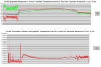
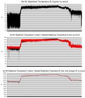
Here a regression polyline (consisting of 20 Kelvin line fragments) using a least squares method for Sol 89 Brightness Temperature B vs. Brightness Temperature A:

It doesn't fully exploit all statistical properties, but it may be useful from a practical point of view as a map from Brightness Temperature B data to an adjusted value comparable to Brightness Temperature A:

The first diagram shows the Sol 89 Brightness Temperature B, as provided by the PDS data.
The second plot shows the adjusted B data (in red) together with A data (in black).
The third diagram shows the two Brightness Temperatures averaged over a 40 record window, respectively. Averaging adjusted B-temperatures should be sufficiently appropriate.

EDIT: Replaced graphics after fixing inaccuracies of the least squares algorithm.