Printable Version of Topic
Click here to view this topic in its original format
Unmanned Spaceflight.com _ Juno _ Juno, perijove 12
Posted by: PhilipTerryGraham Mar 28 2018, 04:10 AM
So, https://www.missionjuno.swri.edu/junocam/voting?current, apparently the spacecraft's being spun around to get the instruments pointed directly at the planet. Io and Ganymede will also be imaged during this pass, as they'll come into view of JunoCam two hours before and twelve hours after closest approach, respectively. For Io, the team are "planning to take two pictures - one exposed nominally and one that over-exposes Io to look for volcanic plumes extending above the surface." The Great Red Spot is also expected to come into view during the spacecraft's departure.

|
Here's a logo for Perijove 12 I threw together, by the way.

Posted by: mcaplinger Apr 3 2018, 12:35 AM
First batch of PJ12 images are available on missionjuno.
It's taking a while since most of the DSN passes are only 40 Kbps.
Posted by: Sean Apr 3 2018, 06:12 AM
PJ12_85
https://flic.kr/p/231X9Yb
Happy Easter indeed.
Posted by: Gerald Apr 3 2018, 06:18 AM
After a long night of PJ12 image processing, the sun is shining again.
First, http://junocam.pictures/gerald/uploads/20180403/.
Now, the JPG version of reprojected images in reverse order:
#086:
|
Posted by: Gerald Apr 3 2018, 06:19 AM
#085:
|
Posted by: Gerald Apr 3 2018, 06:21 AM
#084:
|
Posted by: Gerald Apr 3 2018, 06:23 AM
#082, and #081:
|
|
Posted by: Gerald Apr 3 2018, 06:27 AM
#080, #079, and #077:
|
|
|
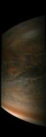
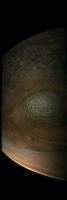
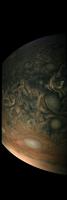
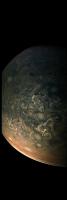
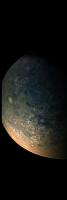
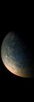
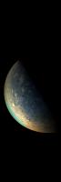
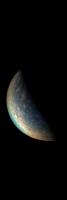
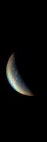
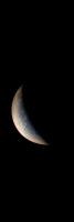
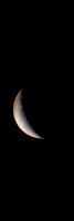
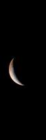
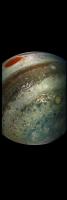
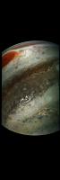
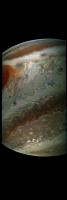
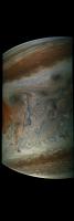
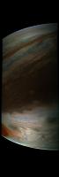
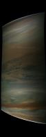
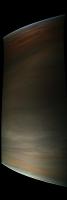
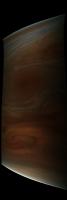
Posted by: Gerald Apr 3 2018, 06:35 AM
#076, #075,
#074, #073,
#072, and #71:
|
|
|
|
|
|
Some of the images have been taken with TDI 3, one with TDI 6, in order to improve S/N for the CPCs (circumpolar cyclones). This caused overexposure of portions of the respective images.
Posted by: Gerald Apr 3 2018, 07:18 AM
http://junocam.pictures/gerald/uploads/20180403a/. The early approach images are white in these renditions due to the percentile-based exposure adjustment applied. I may render smaller crops for the approach sequence later; this will avoid the whitening.
Note the moon shadow in #41.
Posted by: Sean Apr 3 2018, 10:40 AM
PJ12_85 [G.Eichstadt]
Details...
https://flic.kr/p/25HfPyu
https://flic.kr/p/25HfRZS
( processed/blended/edge fills )
Posted by: Sean Apr 3 2018, 08:29 PM
Thanks to Gerald's efforts, here are some PJ12 portraits...
PJ12_Sequence_Part1
https://flic.kr/p/233cvS1
PJ12_80
https://flic.kr/p/HEbLCQ
PJ12_81
https://flic.kr/p/24qVMDc
PJ12_82
https://flic.kr/p/25Je3vj
PJ12_84
https://flic.kr/p/G8TCQg
PJ12_85
https://flic.kr/p/25JdTwN
PJ12_86
https://flic.kr/p/25NaXbn
*Upscaled, white balance, local contrast, repaired, each layer blended & masked ( depending on image content ) before downscaling, consolidating edits.
Posted by: PhilipTerryGraham Apr 4 2018, 05:39 AM
Quick question, what was the distance between the spacecraft and Io when Juno took its pictures of the moon?
Posted by: Brian Swift Apr 4 2018, 07:02 AM

If anyone answers this for Philip, can you also post which spice kernels were loaded to make the determination.
Posted by: mcaplinger Apr 4 2018, 03:03 PM
Using juno_pred_orbit.bsp at webgeocalc, the distance was about 550,000 km.
Posted by: Sean Apr 4 2018, 05:00 PM
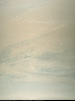
I wondered what size 'Anticyclonic White Oval WS-4' was so I asked astronomer Ronald Drimmel ( @rdrimmel ) on Twitter who referred to Damian Peach's portrait of Jupiter taken the day before Juno's encounter.
We managed to identify the area photographed by Juno from Damien's observation and came away with the answer 'Slightly larger than Earth's Moon'...
https://flic.kr/p/G9SKJc

I've also made some interpolations of Perijove 12 features using Gerald's reprojections...
https://drive.google.com/open?id=1yXMXuU2cKQfohqIcLcTYgYCGmeE-8zBA
https://drive.google.com/open?id=16D6CKX45dSdw5cptrkO4El2gXbtShv4T
Posted by: Gerald Apr 4 2018, 05:34 PM
Btw, here the links to the reprojections Seán used for his wonderful animations:
http://junocam.pictures/gerald/uploads/20180403b/.
http://junocam.pictures/gerald/uploads/20180404/.
In those animations, I think, besides cloud motion, we see evidence for parallax. This would provide us with a geometrical basis to estimate the height of the bright "popup clouds".
Posted by: mcaplinger Apr 4 2018, 05:45 PM
This can be determined directly from the Junocam image to some level of accuracy. The metadata says the s/c altitude for this image was 8681.9 km, so the resolution at nadir is 8681.9*673e-6 = 5.8 km/pixel. WS-4 is about 900 pixels across on its long axis in the raw frames, so that's 5220 km (ignoring perspective effects.)
Posted by: mcaplinger Apr 4 2018, 10:04 PM
The second set of PJ12 images, including the GRS images, are now on missionjuno. The rest of the images continue to come down slowly.
Posted by: Gerald Apr 5 2018, 12:27 AM
http://junocam.pictures/gerald/uploads/20180405/.
I'll upload according JPGs here, in reverse order:
#102, and #101:

|
|
Posted by: Gerald Apr 5 2018, 12:28 AM
#100:
|
Posted by: Gerald Apr 5 2018, 12:29 AM
#99:
|
Posted by: Gerald Apr 5 2018, 12:30 AM
#94:
|
(#95 to #98 are methane band images)
Posted by: Gerald Apr 5 2018, 12:32 AM
#93:
|
#92:
|
Posted by: Gerald Apr 5 2018, 12:34 AM
#91:
|
Posted by: Gerald Apr 5 2018, 12:35 AM
#90:
|
Posted by: Gerald Apr 5 2018, 12:37 AM
#89, and #88:
|
|
Posted by: Gerald Apr 5 2018, 12:41 AM
and #87:
|
Interesting, the small reddish eddies in the latitudes close to the northern and southern edge of the GRS, and of course the extended track of mesoscale waves in #90.
Posted by: Sean Apr 5 2018, 01:05 AM
PJ12_99
https://flic.kr/p/24KmHfJ
https://flic.kr/p/GbdV9Z
...made with Brian Swift's Mathematica pipeline
Posted by: Gerald Apr 5 2018, 02:15 AM
http://junocam.pictures/gerald/uploads/20180405a/, without trajectory data, nor shape model nor with patched camera artifacts, just decompanded and geometrically aligned as if the target would be at infinity. Parameters are according to a heuristics derived from earlier perijoves. No perijove specifics have been used, not even Juno's perijove-specific rotation period. It's instead based on a fixed number of interframe delays per Juno rotation period. Very close-up portions of Jupiter are therefore misaligned.
Next, I'll make an attempt to animate parts of the GRS, and of the accompanying turbulence.
Posted by: Sean Apr 5 2018, 11:06 AM
PJ12_100
https://flic.kr/p/24L5rpm
PJ12_99 Details
https://flic.kr/p/25RjVMz
https://flic.kr/p/Gc6DUt
Posted by: Gerald Apr 5 2018, 01:15 PM
PJ-12 images reprojected to the image stop time of
http://junocam.pictures/gerald/uploads/20180405g/
http://junocam.pictures/gerald/uploads/20180405f/
http://junocam.pictures/gerald/uploads/20180405e/
http://junocam.pictures/gerald/uploads/20180405d/
http://junocam.pictures/gerald/uploads/20180405c/
http://junocam.pictures/gerald/uploads/20180405b/
http://junocam.pictures/gerald/uploads/20180404a/.
An exaple application: Image #092 patched with image #099:
|
I've also submitted to missionjuno a very first attempt to animate the region near the GRS from #092's vantage point.
Posted by: Sean Apr 5 2018, 03:41 PM
Impressive work Gerald... I decided to make a portrait from 3 of your reprojected frames...
https://flic.kr/p/236KHAE
Posted by: JRehling Apr 5 2018, 04:11 PM
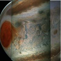
The Great Red Spot has some strikingly and not trivial 3D appearance to my eye. Besides an overall bulge, I see what seems to be a single swirl around the western portion that appears to be at a higher altitude than the other clouds, and/or it swirls outside the rest of the GRS around the ten o'clock position (north=up). In principle, this could all be illusion on an essentially flat (at the given resolution) single layer, but it certainly makes me wonder if, given the right ground truths about how shading and color work, we could reconstruct a good 3D model that would be pretty complex.
We've seen the GRS at better resolution, but this oblique view is really striking even if the 3D I think I see is a trompe l'oeil.
Posted by: Gerald Apr 5 2018, 04:32 PM
First, I'm astonished, how fast Seán was able to compose such a seamless and smooth result.
And yes, from that distance, and far away from the terminator, we can't expect to see an obvious 3D texture. Jupiter's colors sometimes are rather suggestive of 3D structures that cannot be real. I guess, that an SfS algorithm would misinterprete colorization as structure like our human vision does. But nevertheless, there appears to exist evident layering of orangish haze above whitish cloud tops right of the GRS in this image.
Posted by: Sean Apr 6 2018, 02:08 AM
PJ12_94_Detail [G.Eichstadt]
https://flic.kr/p/24vjqVZ
PJ12_90_Details
https://flic.kr/p/238t5dy
https://flic.kr/p/24NgbH3
https://flic.kr/p/25Tp5J2
Posted by: scalbers Apr 6 2018, 04:47 PM
There are variational tomographic methods that can do this sort of thing, at least on Earth as described in this video:
https://www.youtube.com/watch?v=Omoxhoa4iPc
Posted by: Sean Apr 6 2018, 05:22 PM
PJ12_92 [Eichstadt/Doran]
https://flic.kr/p/HKPcj1
https://flic.kr/p/25PSf2S
Posted by: Sean Apr 6 2018, 06:17 PM
Various details from PJ12 [Eichstadt/Doran]
81
https://flic.kr/p/24NEiCu
82
https://flic.kr/p/25PWksy
84
https://flic.kr/p/24NEdLA
85 [patched lower left]
https://flic.kr/p/25PWaTJ
86
https://flic.kr/p/25TLqTt
Posted by: jccwrt Apr 9 2018, 02:15 AM
Some processed images from PJ12
Some really fascinating cloud motions in a region of the North Equatorial Belt:
https://flic.kr/p/25UxiWo
Image taken at perijove - spectacular examples of the small cyclonic systems all over the NEB:
https://flic.kr/p/24B8gwe
Streaky high-altitude clouds and gaps presumably exposing the deeper colorless water vapor cloud deck. The patterns of the surrounding high altitude clouds remind me a lot of transverse cirrus bands that form when convective systems are interacting with jet streams.
https://flic.kr/p/25Uxi9b
Finally, the closest shot of the South Temperate Disturbance. Lots going on here!
https://flic.kr/p/24B8hrF
Posted by: Sean Apr 11 2018, 12:39 AM
PJ12_GRS_reprojected [Eichstadt/Doran]
5 frames blended to produce the following;
https://flic.kr/p/263hW3x
https://flic.kr/p/HUEhaY
https://flic.kr/p/263hWLB
https://flic.kr/p/263hVKP
Data gaps in top left, top right, bottom right corners clone filled/blurred
Posted by: Gerald Apr 11 2018, 01:36 AM
Those are fantastic results, Seán!
This PJ12 flyby is so incredibly rewarding.
...Now better fasten your seat-belts, before you scroll down on this site of
http://junocam.pictures/gerald/uploads/20180410a/.
This preliminary version is also submitted to missionjuno/processing.
I'll need some sleep now, before I'll try to create some refined versions.
Posted by: Gerald Apr 12 2018, 06:53 PM
http://junocam.pictures/gerald/uploads/20180412a/.
Posted by: monty python Apr 16 2018, 05:07 AM
This PJ12 flyby is so incredibly rewarding
This preliminary version is also submitted to missionjuno/processing.
I'll need some sleep now, before I'll try to create some refined versions.
Wonderful and shows the dynamics going on there.
Posted by: Gerald Apr 17 2018, 08:35 AM
https://www.missionjuno.swri.edu/junocam/processing?id=4548, http://junocam.pictures/gerald/uploads/20180416/. I've also added stills of the overexposed northern images, which aren't included into the final MP4 product.
I'll continue to work on some pending maps and cloud animations, today.
Posted by: avisolo Apr 17 2018, 09:04 AM
I'll continue to work on some pending maps and cloud animations, today.
THIS IS ASTONISHING WORK GERALD!!!
Here is my modest reworking of your video, this time with a soundtrack from 'Europa Report' composed by Bear McCreary:
https://vimeo.com/265043136
Please feel free to share:)
Posted by: Sean Apr 17 2018, 05:47 PM
Here is my initial pass on Gerald's excellent animation.
https://flic.kr/p/GBiW3H
Re-timed / Gamma / Sharpen
https://www.youtube.com/watch?v=6DyoK8bdpio
Posted by: Brian Swift Apr 17 2018, 06:11 PM
Perijove 12 in 6 seconds https://youtu.be/3BQgkKr6Q8M processed with Juno28g pipeline.
Posted by: Sean Apr 18 2018, 04:18 PM
For fun I decided to convert a portion of Gerald's PJ12 time-lapse to real time...
https://flic.kr/p/JafohL
https://www.youtube.com/watch?v=oD-1pVDCuvs
The portion rendered in this video occurs between images 93 & 94 in the perijove 12 sequence.
According to Mission Juno metadata, the timestamp difference between these images is 5 minutes 6 seconds.
This information was used to convert the time-lapse portion to real time.
I'm tempted to build a full real time movie from 76 to 102, lasting 1h48m18s!
Posted by: Gerald Apr 18 2018, 04:46 PM
These are the times of the scenes: proc_movie_L3_001_pj12_v01_092_s20_meta.txt ( 2.09K )
: 325
proc_movie_L3_001_pj12_v01_092_s20_meta.txt ( 2.09K )
: 325
Each scene is starting with still image number 0, stills have been rendered in steps of simulated real time 5.0 seconds.
Scene numbers are encoded in the still file names:
File truncs end with the scheme "_xx_nnnnnn_taylorIncEm.bmp_sphC_", with xx the scene number, and nnnnnn the number of the still within the scene, i.e. still image time = RenderStartTime + nnnnnn * 5 sec.
Posted by: Sean Apr 18 2018, 04:55 PM
Does this tally with my understanding of the timings involved Gerald? ( ie does the animation look right to you? )
Posted by: Gerald Apr 18 2018, 05:02 PM
The whole movie would take 2:30:05.000 in real-time, if you start with image #0 of scene #01, and end with the last image of scene #20.
I didn't check your #93 & #94 sequence exactly. But if you're intending to do that load of work, I thought you might be interested in the actual metadata in order to obtain a result as close to real time as possible.
Posted by: Sean Apr 18 2018, 05:26 PM
Thanks for that Gerald, a 2 hour movie would be as good as a shorter one.
I am masking & blending the data gaps with some success, they are quite obvious when shown in time-lapse but would 'disappear' when rendered in real time.
Posted by: Johann Guillon Apr 18 2018, 05:35 PM
I am masking & blending the data gaps with some success, they are quite obvious when shown in time-lapse but would 'disappear' when rendered in real time.
Hi Sean.
Your work is very fine.
I wonder what kind of software do you use to recreate missing frames in an animation.
The result is very impressive on your orbit video.
Thanks for sharing your work with us.
Johann
Posted by: Sean Apr 18 2018, 06:18 PM
Thanks Johann,
I use After Effects with Pixel Warp & Twixtor. The 'Orbit' shots were a challenge because of dirt on ISS windows, since the software does not discern Z axis. I had to 'clean' the windows!
Posted by: Johann Guillon Apr 18 2018, 08:44 PM
I use After Effects with Pixel Warp & Twixtor. The 'Orbit' shots were a challenge because of dirt on ISS windows, since the software does not discern Z axis. I had to 'clean' the windows!
Thanks for the answer.
I watched Eye of Gita, the render is sharp and smooth. Your computer is a monster.
I stop now because it's out of topic.
Very great work once again.
Have a great day !
Posted by: Sean Apr 18 2018, 08:55 PM
Thanks Johann. My PC is fairly mid-range, except with 32gb of ram. 
Here are some real time 2 minute motion portraits of Jupiter thanks to Gerald's original animation and metadata listing. [ test bed for a full perijove 12 real time conversion ]
https://flic.kr/p/25doSp9
https://www.youtube.com/watch?v=CJErniO7rbQ
https://flic.kr/p/25dqeSC
https://www.youtube.com/watch?v=bdUpjr9zEfE
https://flic.kr/p/26iibXH
https://www.youtube.com/watch?v=OzMSLvE65P4
https://flic.kr/p/GDuDy6
https://www.youtube.com/watch?v=F9dPbBWnlxc
https://flic.kr/p/26eLLkW
https://www.youtube.com/watch?v=PSujv9tPSN4
https://flic.kr/p/26irafi
https://www.youtube.com/watch?v=F9iNqCZ4it0
https://flic.kr/p/24Wvyna
https://www.youtube.com/watch?v=s-OL9NjFtLk
Posted by: Sean Apr 21 2018, 08:06 AM
https://www.youtube.com/watch?v=GPMK_6-QrIg
A 2 hour sequence from Gerald's timelapse, trimmed by 30 minutes.
Posted by: Sean May 8 2018, 09:53 AM
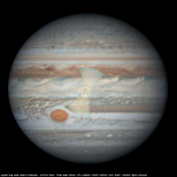
This portrait from Perijove 12 is made by reprojecting 5 separate images [ courtesy of Gerald ] to this viewpoint and blending/healing lots in Photoshop...
https://flic.kr/p/JP2w5Y
Posted by: Sean May 12 2018, 07:16 PM
All the perijoves up to 12 in this updated menagerie...
https://flic.kr/p/27655Za
http://www.gigapan.com/gigapans/208233
Posted by: Gerald May 12 2018, 11:09 PM
Here is a europlanet press release about our ProAm Juno meeting a few days ago:
http://www.europlanet-eu.org/new-views-of-jupiter-showcases-swirling-clouds-on-giant-planet/
Of course my main talk has been only one among several contributions. But Anita Heward, who has written that excellent press release, was especially interested in highlighting Seán's and my JunoCam image products. So, I provided her some of my crazy attempts to infer a vector field of displacements from a pair of reprojected, cropped, contrast-normalized, and heavily enhanced PJ12 JunoCam images.
Besides Seán's latest masterpiece of merging, cleaning, and enhancing some of my reprojections, you'll find an animation, together with a link to an according MP4, in the above article, if you scroll down a bit. It extrapolates one of the two images 100-fold into the past, and into the future, with respect to the time span between the two original images. The morph is an integration assuming a stable velocity field. It's calculated via numerical integration of the numerically given differential equation using probably the simplest-known method, called https://en.wikipedia.org/wiki/Euler_method. I've subdivided either integration into 1,000 equal steps, such that I expected the numerical error being considerably smaller than the statistical and systematic errors, despite the slow convergence behavior of this method.
In order to avoid artifacts induced by regular grids, I've applied Monte Carlo methods whenever I had a choice within the short preparation time.
My full talk considered derivatives like https://en.wikipedia.org/wiki/Vector_calculus_identities, as well as the effect of statistical errors induced by the choice of the actual Monte Carlo samples for stereo correlation.
I might be able to upload the according MP4 (without audio, 630 MB) next weekend, and provide an according link.
Posted by: fredk May 12 2018, 11:27 PM
Congaratulations guys on all this work.
I'm curious, Gerald, which DE did you solve?
Posted by: Gerald May 13 2018, 12:12 AM
Thanks!
The displacement field derived by stereo correlation, and smoothed by a bandpass filter represents a numerical description of a vector field, such that numerical integration methods for differential equations can be applied, especially solutions of the https://en.wikipedia.org/wiki/Initial_value_problem. A morph is essentially such a solution applied to a set of initial values.
At this level of elaboration, the displacement field is just a vector field of pixel displacements, i.e., the displacement is a function of pixel position, however not yet of an immediate physical meaning due to the neglected projection between image coordinates and physically more meaningful coordinates. The differential equations are also only given numerically and implicitely in terms of displacement fields, although some of the derived entities are related to the https://en.wikipedia.org/wiki/Navier%E2%80%93Stokes_equations.
Especially, I've made some experiments with the https://en.wikipedia.org/wiki/Lamb_vector and its first derivative, in order to get an idea, whether a verification of the Navier-Stokes equations might be feasible, or where the velocity field is consistent with the assumption to be https://en.wikipedia.org/wiki/Conservative_vector_field#Irrotational_vector_fields.
Like Anita has written, those are feasibility tests that give a qualtitative idea, not yet final physically calibrated and fully interpreted results.
Posted by: Sean May 15 2018, 10:14 AM
PJ12_81 using Brian Swift's pipeline...
https://flic.kr/p/24qJfPo
*edit: fixed link*
Posted by: Gerald May 17 2018, 02:49 PM
YouTube upload of https://youtu.be/QCGSBk6k9bQ is completed.
And here the original http://junocam.pictures/gerald/talks/europlanet_london_20180510/versions/London2018_Eichstaedt_PJ12_v10.mp4 of about 630 MB.
Posted by: Bjorn Jonsson May 31 2018, 12:28 AM
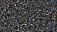
Better late than never; here is an image I processed some time ago from PJ12_90:
|
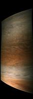
This image has been specially filtered and enhanced to increase the visibility of the mesoscale waves that are present in the pale orange Equatorial Band (EB) within the Equatorial Zone (EZ). Many of waves appear rather subtle if no processing is applied. Bright clouds are also visible near the top of the image. To avoid 'saturating' the bright clouds, the processing of the area containing these clouds differs from the processing elsewhere in the image (in particular, more 'gentle' filtering was used).
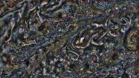
Here is an approximately true color/contrast version:
|
Because of the viewing geometry and the wide field of view the image has some perspective foreshortening. Below is the approximately true color/contrast version with a latitude/longitude grid. Latitude is planetographic.
|
As the latitude/longitude grid implies, the image covers a very small area on Jupiter. A global context view shows this better. It is based on Marco Vedovato's map that includes images from March 29-31, 2018. All of the PJ12_90 observation is shown but the white box shows the extent of the images above:
|
And finally some metadata:
IMAGE_TIME = 2018-04-01T09:52:02.073
MISSION_PHASE_NAME = PERIJOVE 12
PRODUCT_ID = JNCE_2018091_12C00090_V01
SPACECRAFT_ALTITUDE = 4726.4
SPACECRAFT_NAME = JUNO
SUB_SPACECRAFT_LATITUDE = -2.6206
SUB_SPACECRAFT_LONGITUDE = 120.2951
TITLE = Equatorial Zone
Resolution at nadir: ~3.3 km/pixel
Posted by: Gerald May 31 2018, 01:36 AM
For these suble to very subtle features, and for a few other purposes, I've implemented kind of a hipass filter that considers local contrast as well as validity of data.
http://junocam.pictures/gerald/uploads/20180522/JNCE_2018091_12C00090_V01_avrg_Hipass00_taylorIncEm_N_up.png (about 55 MB, 3600x7200 pixels PNG) that averages the hipass-filtered image with an illumination-adjusted and gamma-enhanced version, in order to recover some global colorization.
Rendering large maps with this filter takes several hours, however.
Scroll down to the center and a little further below for the mesoscale waves. There are also some more subtle waves above the center, as well as a second diagonal of wind-blown "popup" clouds, maybe some kind of cirrus, like cirrostratus.
Posted by: fredk Jun 1 2018, 11:59 PM
Sorry, Gerald, I finally looked at those results. It's still not clear exactly what DE you solved. Perhaps you estimated the curl of the initial 2-frame displacement field, and then somehow evolved the field with the constraint that the curl remain constant? So vortices remained localized?
It looks like you also considered the divergence of the initial field, though on physical grounds I guess that should be small in the absence of significant up/downwelling. So any nonzero div may be due to noise in the determination of the initial field, and one approach to reduce noise might be to force the div to zero.
I guess you've made no attempt to try to infer physical quantities such as the pressure field?
Posted by: Gerald Jun 2 2018, 02:47 AM
What I've implemented has been pretty simple. I just inferred a bandpassed displacement field. This could be interpreted as an approximation of a velocity field. Everything is given only numerically.
More generally, this displacement field can be understood as a https://en.wikipedia.org/wiki/Tensor_field, given explicitely.
Each pair (x,y) of the plane is assigned a vector (dx/dt, dy/dt), describing which infinitesimal amount (dx,dy) a vector (x,y) is to be displaced after an infinitesimal time step dt.
Write this assignment as (dx/dt, dy/dt) = f(x,y).
I'd classify this as a https://en.wikipedia.org/wiki/First-order_partial_differential_equation.
So. for each pixel position in the image plane, an approximate velocity is assigned. That's essentially the DE, represented only numerically. This DE can be integrated forward, or backward in time. I've implemented both by the https://en.wikipedia.org/wiki/Euler_method, the most simple numerical method to integrate DEs.
Other than the 1-dimensional case described in Wikipedia, the settings here are 2-dimensional.
And we don't have a time-dependency of the tensor field. It's assumed stable, instead.
All the derivatives are infered numerically from the displacement field (approximate velocity field). They aren't required for the integration of the DE on the above level, but are subject to a separate investigation.
I didn't make assumptions constraining curl, divergence, or Laplace operators, but instead just calculated them numerically from the displacement field. Any assumptions about these operators could be made, but they would define results that should better be determined from the data instead of being presumed. Up and downwelling are well possible and shouldn't be ruled out by assumptions. Even a zero Laplacian may be plausible under idealized conditions. But how can we assume these conditions without trying to measure or infer them? I think, that any unnecessary assumption should be avoided, and we should instead measure and infer everything we can from actual data.
I think, the most significant approach of criticism of the method implemented thus far is the implicite assumption of a stable velocity field. I.e., the integration over the displacement field is assuming, that the displcement field doesn't change over the integration time interval. This simplification, and likely oversimplification, should be verified, at least, or better be refined, by investigating not just a pair of images, but a longer time-series. Such a time series may allow to detect and model changes of the velocity field over time, and result in more accurate particle trajectories than just in flow lines.
Another possibly relevant point is the difficulty to properly determine vectors with a non-zero component normal to Jupiter's "surface", or to the image plane.
Once the numerical representation is fully elaborated, including the reduction to physically meaningful units, this representation can be checked against Navier-Stokes, simplifications to special cases, or extensions.
Posted by: Gerald Jun 2 2018, 11:44 AM
... Example:
Start with the image pair
|
|
...
Posted by: Gerald Jun 2 2018, 11:54 AM
... for each pixel position (x,y), estimate the partial derivatives of x and y with respect to t:
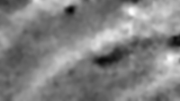
|
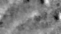
|
That's a visualization of the numerical description of the DE.
Then integrate over time via an Euler method:
 PJ12_099_100_10000samples_mode2_seed000001_grow.mp4 ( 596.69K )
: 233
PJ12_099_100_10000samples_mode2_seed000001_grow.mp4 ( 596.69K )
: 233(here for some randomly chosen initial values)
Posted by: fredk Jun 2 2018, 02:23 PM
Now I see - that is extremely simple. Thanks, Gerald, for the description. So indeed the crucial assumption is of a https://en.wikipedia.org/wiki/Fluid_dynamics#Steady_vs_unsteady_flow, ie constant flow velocity at each point. Indeed looking at more that two frames would help, in at least two ways. First, by giving you a sense of the time dependence of the flow field f(x,y). This could be fitted to simple polynomials or splines to approximate the time dependence (though substantial extrapolation is still risky). But more crucially making several estimates of the flow field would also mean beating down the noise, which has to be large when you only use two frames.
Are there triple or more frame sets that you could use in practice?
My comment about the div wasn't to say you should make that assumption. I think it would simply be interesting to impose div f = 0 and see what difference it makes. A large difference would mean that this is an important consideration and should be investigated further. So it would simply be a test.
Posted by: hendric Jun 2 2018, 03:49 PM
It's like https://earth.nullschool.net/ except for Jupiter! Very nifty!
Posted by: Gerald Jun 2 2018, 05:52 PM
Yes, thanks! That's indeed the same kind of visualization for the flow lines of Earth's wind field.
I guess, that this might be possible closer to the poles. There, we have time series of several images. and may be up to a handfull within a respective series that might be of a sufficient quality to determine velocity fields. During PJ13, for the first time, JunoCam has taken a sequence of TDI 3 images of the south polar region. I think, that those images will be the best basis, thus far, for an attempt to find areas of unsteady flow.
Regarding div, laplace, etc, I've run statistical tests, too, whether the retrieved values are significant, i.e., above noise induced by the choice of Monte Carlo samples used for stereo correspondence. In this repect, all these derived entities appear to deviate significantly from zero, for at least some areas. But there are still statistical errors induced by the structure of the data to be ruled out.
There are various issues to beat down. The first limits I tried to test have been Jupiter's latitude, respectively the time from closest approach. It's the harder to get useful image pairs the closer we get to a perijove. That's due to the very rapid change of perspective. Currently, my limit to get useful results is somewhere near 5 minutes between two images taken from very different perspectives. For the equatorial zone, or later, for the perijove anticipated to migrate towards north, I should push the limits to below two minutes. This requires a very accurate global camera calibration and pointing. Therefore, my primary goal for the next three months is developing families of camera models more suitable for JunoCam calibration than the straightforward Brownian approach.
At the same time, I'll run tests with the south polar PJ13 sequence, in order to be able to provide feedback for planning future flybys (assuming them to take place, and with healthy instruments). One of the tests will include the feasibility of an inference of a displacement field between velocity fields, or at least comparisons between velocity fields derived from image pairs within a sequence of south polar images.
We'll then see, whether or which of those higher-order properties of the velocity field can be determined above noise level.
Posted by: Bjorn Jonsson Jun 2 2018, 06:47 PM
Very interesting discussion, thanks for all of this information
Are there triple or more frame sets that you could use in practice?
I guess, that this might be possible closer to the poles. There, we have time series of several images. and may be up to a handfull within a respective series that might be of a sufficient quality to determine velocity fields. During PJ13, for the first time, JunoCam has taken a sequence of TDI 3 images of the south polar region. I think, that those images will be the best basis, thus far, for an attempt to find areas of unsteady flow.
There are some Voyager triple frame sets where the interval between frames is ~30 minutes if memory serves. It would be interesting to try something like this on these frame sets.
(and now I have yet another reason to be unhappy that Galileo's HGA didn't work...)
Posted by: Gerald Jun 2 2018, 08:41 PM
Agreed, Voyager triplets are definitively worth to be reviewed under this aspect, especially since they could complement for latitudes that are hard to investigate with JunoCam images.
There are also Hubble data that may be feasible for an analysis of mid-scale, short-time dynamics.
The field of applications seems to be much more diverse than I expected after my first tentative experiments.
Posted by: Bjorn Jonsson Jun 16 2018, 12:02 AM
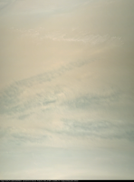
I hadn't yet posted images showing areas north and south of the area shown by my image in http://www.unmannedspaceflight.com/index.php?s=&showtopic=8370&view=findpost&p=239564 so here they are in approximately true color/contrast and enhanced versions:
|
|
|
|
This is processed from PJ12_90.
Posted by: Gerald Aug 11 2018, 04:04 AM
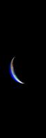
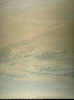
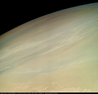
PJ12 #87 seems to show two layers of detached haze:
|
Processing is draft, not reprojected.
Posted by: Sean Aug 16 2018, 01:32 AM
PJ12_80_GE/SD
https://flic.kr/p/27nFUdm
Posted by: Sean Mar 18 2019, 03:42 AM
PJ12_84 revisited
https://flic.kr/p/2dQuSet
Powered by Invision Power Board (http://www.invisionboard.com)
© Invision Power Services (http://www.invisionpower.com)