Printable Version of Topic

Posted by: Kevin Gill Apr 10 2019, 12:06 AM

Looks like a we're limited to the South Pole for PJ19...

https://flic.kr/p/2ftnbce
https://flic.kr/p/2ftnbce

https://flic.kr/p/2enpYQC
https://flic.kr/p/2enpYQC

https://flic.kr/p/2fu63ki
https://flic.kr/p/2fu63ki

https://flic.kr/p/2foGZZS
https://flic.kr/p/2foGZZS

Posted by: mcaplinger Apr 10 2019, 05:23 AM

Yes. The spacecraft was in a different attitude near perijove and we couldn't insure the camera wouldn't image the sun, which could potentially damage it, so we were directed to leave it off.

Posted by: Glenn Orton Apr 10 2019, 11:25 AM

Yes, the spacecraft was turned "sideways" for PJ19 in order for the Microwave Radiometer (MWR) to sweep out a bigger swath of longitude than the nearly "pencil beam" it does on its usual orbits. Both JunoCam and the near-infrared instrument JIRAM were turned off for safety issues, i.e. avoiding pointing into the sun and, for JIRAM, overheating. But they were turned on again once the MWR completed its observations and the spacecraft was again turned back into its normal orientation. The was the first time this approach was used, and there are currently none planned for the remainder of the mission - although that could always change once the full information this mode returned is fully evaluated. -Glenn Orton, Juno science team member

Posted by: Kevin Gill Apr 10 2019, 10:19 PM

Thank you. Seems like a good reason to not use JunoCam. I hope some good science comes out of it.

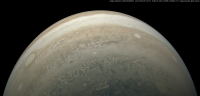
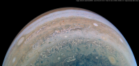
Here's an overview of Perijove 19:

https://flic.kr/p/TmpC4s
https://flic.kr/p/TmpC4s

Posted by: Bjorn Jonsson Apr 10 2019, 10:46 PM

This is image PJ19_1. First an approximately true color/contrast image and then a version with increased contrast that has also been processed to show color differences more clearly:

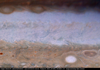
As John Rogers mentions https://www.missionjuno.swri.edu/junocam/processing?id=6782, three small vortices can be seen in the currently whitened South Temperate Belt in the new JunoCam images. Below is a heavily processed map-projected image that shows these ovals:

Posted by: Brian Swift Jan 3 2020, 04:35 AM

Gerald, your "weather forecast" GIF on missionjuno is very cool. A few questions, because I'm a curious cat...
Did you develop your own fluid dynamic simulation or are you using some other CFD software?
What is the simulation time step?
What are the grid dimensions?

Posted by: Gerald Jan 4 2020, 04:19 AM

Thanks, Brian!
I'm developing my own https://en.wikipedia.org/wiki/Computational_fluid_dynamics from scratch, but stuff is non-trivial, so I'm serving myself of the shoulders of giants from a methodological point of view. Like in many other cases, you can really understand things only, if you implement them yourself. Better if you even develop the required methods yourself, and go through all the flaws and glitches you can make. The time step in https://www.missionjuno.swri.edu/Vault/VaultOutput?VaultID=25100&t=1557760266 I've submitted to missionjuno is 1 hour, but the full version is calculated with fixed steps of 6 minutes. In order to keep the file size within reasonable limits, I've taken just each 10th image, and reduced it by a factor of 2. The method is grid-free on an inviscid flat 2D https://en.wikipedia.org/wiki/Biot%E2%80%93Savart_law approach with a https://en.wikipedia.org/wiki/Stream_function-derived 2D https://en.wikipedia.org/wiki/Vorticity field of the south polar region of PJ19 as initial condition of an initial value problem. Algorithmic complexity is O(tn²), with n the number of 4th order "Gauss-https://en.wikipedia.org/wiki/Mollifier" "https://en.wikipedia.org/wiki/Dirac_delta_function" and t the number of time-steps. I'm using single-step multi-stage explicit https://en.wikipedia.org/wiki/Runge%E2%80%93Kutta_methods with fixed time-steps of order 4 or 5 for numerical integration of the ODEs. https://en.wikipedia.org/wiki/Dormand%E2%80%93Prince_method are useful to test for the quality of the convergence of the integration.
I'm working on a https://en.wikipedia.org/wiki/N-sphere version in order to get a little more realistic. Simulating on the precise IAU Jupiter 2-spheroid might be algorithmically expensive, and difficult to implement, because of the according https://archive.lib.msu.edu/crcmath/math/math/o/o004.htm. I'm exploring how far I can go within reasonable computational and implementation costs. Even the 2-sphere simulation is much slower(but still O(tn²)) than the flat euclidean 2D plane.
There is much more to tell, maybe within a presentation on one of the conferences this year, provided I'll get an abstract submitted in time.

https://en.wikipedia.org/wiki/Finite_volume_method on a grid appear less suitable in a very turbulent regime. They tend to get numerically unstable for large https://en.wikipedia.org/wiki/Reynolds_number unless very short time steps are applied (see https://en.wikipedia.org/wiki/Von_Neumann_stability_analysis).

Some simulations of turbulence favor https://ethos.bl.uk/OrderDetails.do?uin=uk.bl.ethos.451452. I've still to decide, whether I'll test this family of methods, too. But those hybrid methods are more difficult to understand, and I'm not yet quite sure, whether I'd been able to modify the required https://en.wikipedia.org/wiki/Discrete_Poisson_equation for non-euclidean geometry within short time, if necessary. So, my first choice is the above approach, which I already understand sufficiently well to modify it according to my requirements.

If you are interested in a good introductory paper, I'd recommend https://www.cse-lab.ethz.ch/wp-content/papercite-data/pdf/cottet2000b.pdf.

Posted by: Gerald May 7 2020, 04:49 PM

A more complete answer is online now on the EGU2020 website, including an explanation video at the end of the abstract:
https://meetingorganizer.copernicus.org/EGU2020/displays/36509
Thanks to excellent suggestions of my co-authors Candy and Glenn, and of John Rogers, I hope that the video is of an acceptable quality in the meanwhile. Obviously, further work is TBD.
I first tried to work with a more recent PJ. But PJ19 seems still to be the best JunoCam image sequence to analyse south polar dynamics.
You might imagine, why I didn't find much time for discussions the recent few months