Juno perijoves 2 and 3, October 19 and December 11, 2016 Options

[Brian Swift]

... 'blinking' the red/green/blue channels rapidly in high contrast areas.

Doh. I should have already been doing this. I've just been looking at bue/red fringing in high contrast areas.

Björn, are you using the standard camera model, or have you developed your own?

[Bjorn Jonsson]

Björn, are you using the standard camera model, or have you developed your own?

This depends on how you define "...using the standard camera model" . I'm using software written by myself for the geometric processing (reprojecting the framelets to a simple cylindrical and/or polar map etc.). However, some of the code is directly based on information/code from the IK kernel, in particular the distort/undistort code, the location of R/G/B on the CCD, the FOV etc.. I'm also using the SPICE toolkit. Works wonderfully now, especially after lots of improvements I did in November and December 2019 (what was supposed to be a minor improvement in early November triggered a flood of new ideas for improving the software, resulting in faster processing, improved/proper flatfielding, a new (?) function for removing limb darkening, better photometric parameters, an empirical model of the skylight illumination near the terminator, easier limb fits etc.).

The only issue I'm working on now is the value I need to add to START_TIME. Using a fairly large sample of images it has become absolutely clear that in my case the average value I need to use is lower than the correct value (0.068). The average value I use is close to 0.040 but it varies and is sometimes close to 0.068. This means that something is wrong. This has no visual effect though and is in that sense not a serious problem (in particular there is negligible misalignment between the R/G/B channels or adjacent framelets from the same color channel). I can think of at least three plausible reasons for this (in fact all of them might contribute to the error) and now that I'm almost finished with the PJ24 images (at least for the time being) I plan on taking a detailed look at this issue.

[Brian Swift]

... some of the code is directly based on information/code from the IK kernel, in particular the distort/undistort code,

That is what I was I was referring to. I and (I believe) Gerrald have our own distort/undistort code, Kevin (I believe) is using the standard code via ISIS,
but I didn't know if you had your own or used the standard code.

... in faster processing, improved/proper flatfielding, a new (?) function for removing limb darkening, better photometric parameters, an empirical model of the skylight illumination near the terminator, easier limb fits etc.).

Awesome. Wish I had time to do a proper illumination removal model. When you combine multiple images, is there residual brightness variation that needs to be adjusted to eliminate
boundaries between images?

The only issue I'm working on now is the value I need to add to START_TIME. Using a fairly large sample of images it has become absolutely clear that in my case the average value I need to use is lower than the correct value (0.068). The average value I use is close to 0.040 but it varies and is sometimes close to 0.068.

Note, the START_TIME_BIAS in juno_junocam_v03.ti is 0.06188 not .0688.
My start times (based on limb fit) range from .03 to .08

[Gerald]

That is what I was I was referring to. I and (I believe) Gerrald have our own distort/undistort code...

Yes, so it is. I've implemented almost everything from scratch down to pixel operations in RAM or basic 3D libraries. The only essential thing I didn't implement for JunoCam images is the determination of the s/c trajectory from images. Instead, I'm using the NAIF/SPICE spy.exe utility to save trajectory data to text files. And for movie productions or image file conversions I'm usually making use of ffmpeg. (I've worked on reading some of the image file formats professionally on a binary level for long enough, so that stuff is less interesting from my point of view.)

[Spoiler alert: Don't follow the links below, if you are ambitious to find your own solutions independently.]
During EPCS2018, I explained one of several possible approaches of in-flight geometrical camera calibration on the basis of Marbe Movie images:
PDF version
PPT version (with animations)
In contrast to some of the JunoCam IK documentation, I'm working with the CCD pixel layout. One advantage is the easy adjustment to the changing position of the readout region for the methane band images by 90 pixels. But otherwise, the more recent IKs (instrument kernels) are looking good.

My assumptions about camera pointing are imperfect, and I'm doing some manual limb fitting of each image. But any significant reduction of manual work would only be achieved, if automated pointing data would be better than manual adjustment is able to do. So, further refinement of automated pointing currently isn't my top priority.

And here links to an EPSC2017 talk about polynomial illumination adjustment over the cosines of the incidence and the emission angle:
PDF version
PPT version
There is still some space for further improvements. I might prepare such a solution for EPSC2020, if time allows. Note also, that Jupiter's appearance is changing, and so are best-fit illumination models. But my current focus is on understanding the dynamics of the atmosphere. I presume, that this will also be required for an accurate understanding of light scattering and according models. So, there is significant effort in software development and test runs, and less time for discussions. Some of the results may be worth to be released in formal journal papers, the preparation of which is taking time, too. As usual, I'm interested in in-depth understanding of all theoretical, methodological and technical detail as seamlessly as possible. And learning means inventing, or re-inventing, if partial solutions do already exist.

Regarding the limb fit: Note, that the opacity of the hazes, and so the apparent limb, is varying with latitude. This applies to Jupiter's equipotential wrt to a spheroid, too. (AFAIK, full detail of the latter isn't publicly accessible, yet.)

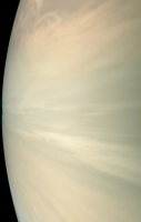
[Bjorn Jonsson]

... in faster processing, improved/proper flatfielding, a new (?) function for removing limb darkening, better photometric parameters, an empirical model of the skylight illumination near the terminator, easier limb fits etc.).

Awesome. Wish I had time to do a proper illumination removal model. When you combine multiple images, is there residual brightness variation that needs to be adjusted to eliminate boundaries between images?

Yes, there are always some differences and I don't think they can ever be eliminated. The reason is that the photometric parameters differ a bit for different parts of Jupiter (in particular I'm pretty sure that the parameters for the polar areas differ from the parameters closer to the equator) and they also vary as a function of time (changes in color/brightness/haze etc.), in other words: There's no such thing as a 'perfect' photometric model for Jupiter. For simplification purposes I'm using the same parameters everywhere.

That said, the differences at the boundaries between images are much smaller now than they used to be when mosaicking images. Of course the intensity differences are smaller but what's maybe even more important is that there are now no significant color differences at the seams (unless there are significant differences in the emission angle).

These smaller differences are not only because of more accurate photometric parameters when removing the illumination effects. I recently discovered that proper and accurate flat fielding is much more important when processing JunoCam images than I used to think. There is some vignetting in the raw images. The effects of flat fielding are not very noticeable in images with lots of high frequency, high contrast features but they are more noticeable in low contrast areas. Here is an image where the effects of flat fielding are particularly noticeable, an animated GIF example from image PJ14_26 (here the illumination has not been changed):



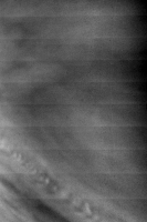
Needless to say the flat fielded images with illumination removed are easier to deal with when making mosaics. The flat fielding also greatly reduces the horizontal banding seen in some images, especially in the blue channel in hi-res images of low contrast areas. This is an example from the blue channel in image PJ10_28 without flat fielding. The contrast has been increased a lot:



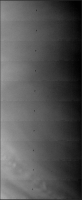
The individual framelets are too dark at the top and too bright at the bottom. Flat fielding greatly reduces this banding but does not completely eliminate it.

The absence of an 'official' JunoCam flat field turned out to be a smaller problem than I was initially expecting. As a starting point I found a flat field image in this post from Mike. Using this image directly didn't work well (I tried all decompanded and not decompanded combinations to be sure). I had to make significant modifications to it in order for it to work well. This was largely a trial and error process involving mosaics where the difference in emission angle is small in the overlap area, checking images where I knew that the brightness near the right edge shouldn't be lower than near the center and also by checking for the horizontal banding mentioned above. I ended up with a flat field that seems to work very well but I'll probably make further modifications to it later - importantly I really have no idea exactly how close it is to a 'perfect' flat field. This is the flat field I'm currrently using:



Apart from other changes, high frequency artifacts, blemishes etc. have been removed since I prefer to fix these in a separate processing step and not as part of the flat fielding.

Has anyone else been flat fielding the JunoCam images and if so, how?

Note, the START_TIME_BIAS in juno_junocam_v03.ti is 0.06188 not .0688.
My start times (based on limb fit) range from .03 to .08

Oops, I didn't look up the correct value before writing the incorrect value 0.068 but it doesn't change the fact that the ~0.040 value I mentioned is suspiciously low. The range I have seen (also from limb fits) is slightly bigger, ~0.005 to ~0.085.

My assumptions about camera pointing are imperfect, and I'm doing some manual limb fitting of each image.
...
Regarding the limb fit: Note, that the opacity of the hazes, and so the apparent limb, is varying with latitude. This applies to Jupiter's equipotential wrt to a spheroid, too. (AFAIK, full detail of the latter isn't publicly accessible, yet.)

I'm also measuring the limb position in every image I process - I've sometimes had the impression that this was rare. I then feed the measured limb positions into software that gives me the START_TIME and interframe delay that are consistent with the measured limb positions. Hazes, variable cloud altitudes etc. greatly complicate this though. Also the appearance of the limb in the blue images is significantly different from the red (and also green) images and this affects the limb position measurements. Maybe I should measure the limb positions from red images only.

[Brian Swift]

Has anyone else been flat fielding the JunoCam images and if so, how?

My flat fields (gains) were derived from average of 150 bright framelets (30 from each of PJ12 to PJ16)
which are smoothed by fitting with a 10th order polynomial. Dark spots in average are merged into
the polynomial based flat.

I've uploaded to GitHub depot the gain, flat (not used), and debias images as 32-bit tiff. https://github.com/BrianSwift/JunoCam/tree/master/Juno3D

An animated gif showing effect of flat field on PJ10_28 blue channel

... I then feed the measured limb positions into software that gives me the START_TIME and interframe delay that are consistent with the measured limb positions.

I only use limb fits to adjust START_TIME. Centering the SPICE limb within the visible limb using average of time offset computed independently for R,G,B.
I assume variance in altitude of visible limb is due to real atmospheric variation relative to the SPICE ellipsoid.
I'm unaware of any physical justification for varying interframe delay.

[Brian Swift]

And here links to an EPSC2017 talk about polynomial illumination adjustment over the cosines of the incidence and the emission angle:

What you discuss in the slides is what I've though about implementing. Though I want the BRDF to extend into the night side past the SPICE terminator,
and to also use data from multiple perijoves.
I also have a concern about the effects of the internal camera light scattering (which I know you've investigated) on the illumination model.

Regarding the limb fit: Note, that the opacity of the hazes, and so the apparent limb, is varying with latitude. This applies to Jupiter's equipotential wrt to a spheroid, too. (AFAIK, full detail of the latter isn't publicly accessible, yet.)

I wonder if there will be any public update to gravity field parameters before the mission concludes.
https://ssd.jpl.nasa.gov/?gravity_fields_op shows 2013 being the last update.

[Gerald]

I wonder if there will be any public update to gravity field parameters before the mission concludes.
https://ssd.jpl.nasa.gov/?gravity_fields_op shows 2013 being the last update.

Considerably improved data have already been published, e.g. 2018 in Nature, "Measurement of Jupiter’s asymmetric gravity field", by Iess & al (paywalled).
Measurements are ongoing. So, I'd presume, that there will be updates released publicly in due time.

Regarding the illumination model: I've also run versions with other PJs than PJ06, or over more than one PJ. PJ06 worked pretty well for several PJs, but for the more recent PJs with very different observational conditions, I've determined some new models. I'm also intending to derive a model suitable for all PJs. But there will be limitations, since Jupiter itself is changing, and its atmospheric properties vary with the location you are looking at. Behind the terminator, it's even worse, since there may or may not be light scattering high-altitude hazes. Hence a perfect illumination model may not exist.
Note also, that higher-order polynomials tend to oscillate and won't improve the results. So, it might be worth to investigate several more families of functions. I've done so to some degree, but didn't make each investigation public. I hope that I'll be able to resume a deeper analysis later this year. I share your concerns about flat fields and various kinds of camera artifacts. All those effects need to be considered and discussed in a paper with a certain science value, especially since we then go beyond the camera design requirements.

[Bjorn Jonsson]

I only use limb fits to adjust START_TIME. Centering the SPICE limb within the visible limb using average of time offset computed independently for R,G,B.
I assume variance in altitude of visible limb is due to real atmospheric variation relative to the SPICE ellipsoid.
I'm unaware of any physical justification for varying interframe delay.

The problem with only adjusting the START_TIME is that then you need to either adjust the Jovian ellipsoid dimensions or the interframe delay. Otherwise you'll probably end up with a small error at the 'lower' limb - therefore I use limb fits at both the 'upper' and 'lower' limb. There probably really isn't any physical justification for adjusting the interframe delay using a significantly lower or higher value than 1 ms. Using e.g. 1.1 ms is probably OK but to me e.g. 0.7 or 1.3 ms is suspicious. I nevertheless often use values as low as ~0.7 or as high as ~1.3 ms (occasionally even lower/higher), mainly as a quick and dirty way to make the position of the 'lower' limb consistent with the position of the 'upper' limb without adjusting the ellipsoid dimensions which is more complicated and might also be incorrect because different cloud deck (or haze) altitudes might be a part of the problem. That said, I suspect the deviations are too big to be caused entirely by cloud/haze variability.

I've uploaded to GitHub depot the gain, flat (not used), and debias images as 32-bit tiff.

Thanks - really interesting. For comparison I'll upload a bias file constructed from PJ8 images in a day or two. It's similar but some of the vertical lines are fainter (or missing) in my bias file.

Exactly how are you using the gainSmooth12to16.tiff file?

[Brian Swift]

Exactly how are you using the gainSmooth12to16.tiff file?

Schematically,
corrected segment = gain * (raw segment - debias)
which I got from https://en.wikipedia.org/wiki/Flat-field_correction

gainSmooth12to16.tiff contains the gain values used for the Blue, Green, and then Red filters ordered from top to bottom.
Values are 32-bit float and can be greater than 1.

Technically, gainSmooth12to16.tiff isn't used by my pipeline.
The gains are embedded in the Mathematica notebook that implements the pipeline.
They are an Association with filter names as the keys and the individual gain images as the values.
I exported them to gainSmooth12to16.tiff to make them more accessible to other developers.

This is the Mathematica code that implements the entire flat-field operation:

CODE

flatFieldCorrect[rawFramlet_Image, chanKey_] := ImageMultiply[
  ImageSubtract[rawFramlet, debias[[chanKey]]], gain[[chanKey]]]

flatFieldCorrectSegments[segments_Association] := MapIndexed[
  Function[{framelets, filter},
   Map[flatFieldCorrect[#, filter[[1]]] &, framelets, {2}]
   ]
  , segments]

[Brian Swift]

...you need to either adjust the Jovian ellipsoid dimensions or the interframe delay. Otherwise you'll probably end up with a small error at the 'lower' limb ...

Are you basically stating you need to adjust the ellipsoid dimensions or the interframe delay to get all the Junocam imagery to "fit" onto the SPICE ellipsoid?

If so, it hasn't been an issue for my pipeline, since it can map raw imagery that doesn't project onto the ellipsoid to the (non map projected) output image.

[Bjorn Jonsson]

Are you basically stating you need to adjust the ellipsoid dimensions or the interframe delay to get all the Junocam imagery to "fit" onto the SPICE ellipsoid?

If so, it hasn't been an issue for my pipeline, since it can map raw imagery that doesn't project onto the ellipsoid to the (non map projected) output image.

Strictly speaking, yes. However, the error is small so you can probably safely omit this in most cases - also you are mapping the raw imagery that doesn't project onto the ellipsoid to the output image so this is less important in your case. The reason I'm doing this is that I usually want very high accuracy at the limb. I want to avoid 'truncating' the limb (or getting an extended almost black area outside of the limb). To get really high quality results at the limb (haze layers and bluish sky) I sometimes add 200 km to the ellipsoid radii, both when reprojecting the images to simple cylindrical maps and when rendering the maps in a 3D renderer.

[mcaplinger]

There probably really isn't any physical justification for adjusting the interframe delay using a significantly lower or higher value than 1 ms. Using e.g. 1.1 ms is probably OK but to me e.g. 0.7 or 1.3 ms is suspicious.

The 1 msec is simply a fixed command offset we forgot to account for.

The clock oscillator that is commanding the frames is advertised as being +/- 150 PPM over its entire temperature range and radiation dose. So changing the typical interframe of 370 msec by more than about 55 microseconds would mean the oscillator is not performing to specifications. Which is certainly possible, but I would expect some systematics we're not seeing were it the case.

We are in the process of releasing revised START_TIMES to the PDS based on manual measurement of the first limb crossing. There could be many explanations of what might cause mismatches at the last limb crossing (interframe off, spin axis or rate knowledge off, speed of light not being properly accounted for, deviation of limb from spheroid, etc.) My goal has merely been to get to the point where the community can use ISIS3 without seeing unacceptably large inconsistencies, and I think we've achieved that.

[Bjorn Jonsson]

The clock oscillator that is commanding the frames is advertised as being +/- 150 PPM over its entire temperature range and radiation dose. So changing the typical interframe of 370 msec by more than about 55 microseconds would mean the oscillator is not performing to specifications. Which is certainly possible, but I would expect some systematics we're not seeing were it the case.

This is consistent with what I saw when processing an EFB image several weeks ago. In that case the value I had to add was the expected 1 ms. I got worse results when I got curious and tested other values, including values 'very' close to 1 ms (e.g. 0.95 or 1.05). Of course the difference here is that the target body dimensions are precisely known and limb fits are also easier since I have better knowledge of how clouds/hazes behave at the limb in images of the Earth.

[Bjorn Jonsson]

For comparison I'll upload a bias file constructed from PJ8 images in a day or two. It's similar but some of the vertical lines are fainter (or missing) in my bias file.

And here it is, a contrast enhanced bias file constructed from 57 PJ8 R/G/B framelet sets:



And this is a contrast enhanced version of the bias file posted above by Brian:


Interestingly, some of the vertical lines are missing in my PJ8 bias image. Other features are similar.